Continuous Distribution Functions
Continuous Distribution Functions. Jake Blanchard Spring 2010. The Normal Distribution. This is probably the most famous of all distributions At one time, many felt that this was the underlying distribution of nature and that it would govern all measurements

Continuous Distribution Functions
E N D
Presentation Transcript
Continuous Distribution Functions Jake Blanchard Spring 2010 Uncertainty Analysis for Engineers
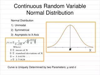
The Normal Distribution • This is probably the most famous of all distributions • At one time, many felt that this was the underlying distribution of nature and that it would govern all measurements • It is also called the Gaussian distribution • Many random variables are not well-represented by this distribution, so its popularity is not always warranted • Since limits are +/- infinity, this distribution is problematic in some situations Uncertainty Analysis for Engineers
For Example • Suppose we measure the height of many people and want to represent the data with a normal distribution • Obviously, the distribution will predict a finite probability for negative heights, which makes no sense • On the other hand, a height of 0 will be several standard deviations from the mean, so the error will be negligible • In some cases, we can just truncate the predictions Uncertainty Analysis for Engineers
Normal distribution Uncertainty Analysis for Engineers
Central Limit Theorem • One of the key reasons the normal distribution is the CLT • It states that the distribution of the mean of n independent observations from any distribution with finite mean and variance will approach a normal distribution for large n Uncertainty Analysis for Engineers
Examples • Here are some examples of phenomena that are believed to follow normal distributions • Particle velocities in a gas • Scores on intelligence tests • Average temperatures in a particular location • Random electrical noise • Instrumentation error Uncertainty Analysis for Engineers
The Half-Normal Distribution • Useful when we are interested in deviations from the mean Uncertainty Analysis for Engineers
Half-Normal Distribution Uncertainty Analysis for Engineers
When would we use this? • Suppose we build a flywheel from two parts. • It is important that they be nearly the same weight • We measure only the difference in weight • This will be positive and is likely to be normally distributed, with the bulk of the results near 0 • The half-normal distribution should work Uncertainty Analysis for Engineers
Bivariate Normal Distribution • Joint distribution Uncertainty Analysis for Engineers
What if x and y are not correlated? • The correlation coefficient will be 0 • The joint pdf becomes the product of two separate normal distributions and x and y can be considered independent • Be careful, lack of correlation does not always imply independence Uncertainty Analysis for Engineers
The Gamma Distribution • For random variables bounded at one end • Peak is at x=0 for less than or equal to 1 • CDF is known as incomplete gamma function Uncertainty Analysis for Engineers
Gamma distribution Uncertainty Analysis for Engineers
Facts on Gamma Distribution • Appropriate for time required for a total of exactly independent events to take place if events occur at a constant rate 1/ • Has been used for storm durations, time between storms, downtime for offsite power supplies (nuclear) Uncertainty Analysis for Engineers
Examples • If a part is ordered in lots of size and demand for individual parts is 1/ , then time between depletions is gamma • System time to failure is gamma if system failure occurs as soon as exactly sub-failures have taken place and sub-failures occur at the rate 1/ • The time between maintenance operations of an instrument that needs recalibration after uses is gamma under appropriate conditions • Some phenomena, such as capacitor failure and family income are empirically gamma, though not theoretically Uncertainty Analysis for Engineers
Practice • A ferry boat departs for a trip across a river as soon as exactly 9 cars are loaded. Cars arrive independently at a rate of 6 per hour. What is probability that the time between consecutive trips will be less than one hour? What is the time between departures that has a 1% probability of being exceeded? Uncertainty Analysis for Engineers
Solution • Time between departures is gamma. • =9 cars, 1/ =6 per hour • Evaluate F(1) numerically • Matlab • gamcdf(1,9,1/6) • F=0.153 • Or • f=@(x) x.^8.*exp(-6*x) • 6^9/gamma(9)*quad(f,0,1) Uncertainty Analysis for Engineers
Solution continued • Solve this for x • gaminv(0.99,9,1/6) • Solution is x=2.9 hours • That is, the chances are 1 in 100 that the time between departures will exceed 2.9 hours Uncertainty Analysis for Engineers
Generalized gamma distribution • We can redefine the gamma distribution to be 0 below some value () Uncertainty Analysis for Engineers
Exponential Distribution • This is just a gamma distribution with =1 and =1/ Uncertainty Analysis for Engineers
Exponential distribution Uncertainty Analysis for Engineers
Facts (Exp Distribution) • Useful for time interval between successive, random, independent events that occur at constant rates • Time between equipment failures, accidents, storms, etc. • Given our discussion of the gamma distribution, this distribution is a good model for the time for a single outcome to take places if events occur independently at a constant rate Uncertainty Analysis for Engineers
Example • If particles arrive independently at a counter at a rate of 2 per second, what is the probability that a particle will arrive in 1 second? • =2 • F(1)=1-exp(-2*1)=0.865 Uncertainty Analysis for Engineers
Beta Distributions • This is useful when x is bounded on both ends • x is bounded between 0 and 1 • f can be u-shaped, single-peaked, J-shaped, etc. • The CDF is the incomplete beta function Uncertainty Analysis for Engineers
Beta distribution Uncertainty Analysis for Engineers
Facts (Beta Distribution) • The many shapes this distribution can take on make it quite versatile • Often used to represent judgments about uncertainty • Can be used to represent fraction of time individuals spend engaging in various activities • …or fraction of time soil is available for dermal contact by humans (as opposed to being covered by soil and ice) • …or fraction of time individual spends indoors Uncertainty Analysis for Engineers
More Examples • A measuring device allows the lengths of only the shortest and longest units in a sample to be recorded. 15 units are selected at random from a large lot. What is the probability that at least 90% have lot lengths between the recorded values? • 20 electron tubes are tested until, at time t, the first one fails. What is the probability that at least 75% of the tubes will survive beyond t? Here, 1=1 and 2=0 Uncertainty Analysis for Engineers
Uniform Distribution • Actually a special case of the beta distribution (1=1 and 2=1) Uncertainty Analysis for Engineers
Uniform distribution Uncertainty Analysis for Engineers
Lognormal Distribution • The natural log of the random variable follows a normal distribution • It can be modified to be 0 before some non-zero value of x Uncertainty Analysis for Engineers
Lognormal Distribution • It can be used as a model for a process whose value results from the multiplication of many small errors in a manner similar to the addition of many instances we discussed with respect to the normal distribution • The product of n independent, positive variates approaches a log-normal distribution for large n Uncertainty Analysis for Engineers
Lognormal distribution Uncertainty Analysis for Engineers
Lognormal facts • Good for • chemical concentrations in the environment, deterioration of engineered systems, etc. • asymmetric uncertainties • processes where observed value is random proportion of previous value • It is “tail-heavy” Uncertainty Analysis for Engineers
Examples • Distribution of personal incomes • Distribution of size of organism whose growth is subject to many small impulses, the effect of each being proportional to the instantaneous size • Distribution of particle sizes from breakage Uncertainty Analysis for Engineers
Statistical Models in Life Testing • Time-to-failure models are a common application of probability distributions • We can define a hazard function as • where f and F are the pdf and CDF for the time to failure, respectively • h(t)dt represents the proportion of items surviving at time t that fail at time t+dt Uncertainty Analysis for Engineers
Hazard Functions • A typical hazard function is the so-called bathtub curve, which is high at the beginning and end of the life cycle • Uniform distribution – U(0,1) • Exponential distribution Probability of failure during a specified interval is constant Uncertainty Analysis for Engineers
Weibull Distribution • This is a generalization of the exponential distribution, but, for time-to-failure problems, the probability of failure is not constant Uncertainty Analysis for Engineers
Weibull distribution Uncertainty Analysis for Engineers
Weibull Facts • Useful for time to completion or time to failure • Can skew negative or positive • Less tail-heavy than lognormal Uncertainty Analysis for Engineers
Extreme Value Distributions • Here we are interested in the distribution of the “largest” or “smallest” element in a group • For example, • What is the largest wind gust an airplane can expect? Uncertainty Analysis for Engineers
Types of EV Distributions • Type I (Gumbel) for maximum values • Type1 (Gumbel) for minimum values • Type III (Weibull) for minimum values Uncertainty Analysis for Engineers
The Gumbel Distribution • Limiting model as n approaches infinity for the distribution of the maximum of n independent values from an initial distribution whose right tail is unbounded and is “exponential” • original distribution could be exponential, normal, lognormal, gamma, etc. – all have proper characteristics Uncertainty Analysis for Engineers
Type I EV • Can represent • Time to failure of circuit with n elements in parallel • Yearly maximum of daily water discharges for a particular river at a particular point • Yearly maximum of the Dow Jones Index • Deepest corrosion pit expected in a metal exposed to a corrosive liquid for a given time? Uncertainty Analysis for Engineers
Type I (Gumbel) Uncertainty Analysis for Engineers
Gumbel distribution Uncertainty Analysis for Engineers
Example • The maximum demand for electric power at any time during a year in a given locality is related to extreme weather conditions • Assume it follows a Type 1 distribution with L=2000 kW and =1000 kW. • A power station needs to know the probability that demand will exceed 4000 kW at any time in a year and the demand that has only a 1/20 probability of being exceeded in a year Uncertainty Analysis for Engineers
Solution • evcdf(4000,2000,1000) • =0.9994 • For second part, solve F(y)=0.95 for y • evinv(0.95,2000,1000) • Result is 3097 kW Uncertainty Analysis for Engineers
Type III • This is the Weibull distribution • It is the limiting model as n approaches infinity for the distribution of the minimum of n values from various distributions bounded at the left • The gamma distribution is an example • For example, a circuit with components in series with individual failure distributions that are gamma, then the Type III EV distribution is appropriate Uncertainty Analysis for Engineers
Other examples • Failure strength of materials • Drought analyses Uncertainty Analysis for Engineers
Observations • The log of the weibull distribution is distributed as a minimum value Type I • These extreme value distributions are only valid in the limit of large n – convergence depends on initial distributions • 10 samples can be adequate for initial distributions that are exponential • It may take as many as 100 for normal distributions Uncertainty Analysis for Engineers