Continuous Probability Distribution
This comprehensive guide covers key concepts in continuous probability distributions, focusing on the attributes of continuous random variables, including the Uniform and Normal distributions. We explain the Probability Density Function (PDF) and how it reflects probabilities through areas. The guide further elaborates on the significance of the Central Limit Theorem (CLT) in sampling distributions, emphasizing how sample means tend to be normally distributed. Learn about standardization and how to utilize percentiles effectively for statistical inference.

Continuous Probability Distribution
E N D
Presentation Transcript
Continuous Probability Distribution • A continuous random variables (RV) has infinitely many possible outcomes • Probability is conveyed for a range of values, not for individual values. • Example: Satellite falling from orbit. • Uniform Probability Distribution • All outcomes are equally likely. • Shape of distribution is a rectangle.
Probability Density Function (PDF) • A PDF is used to convey probability for a continuous random variable. • Area under the PDF indicates probability • Total area under the PDF is 1 • The PDF must be non-negative for all values • The probability of an observation falling between a and b is equal to the area under the PDF between a and b.
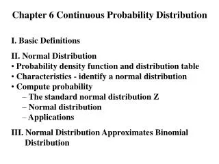
Normal (Gaussian) Distribution • Many real world applications utilize the normal distribution. • Naturally occurs in test scores, experimental errors, measures of sizes in populations, etc. • Data that is summed or averaged can be shown to follow a distribution.
µ Normal Probability Distribution • PDF: • Shape: • Bell-Shaped and Symmetric • Mean, median and mode are equal
Normal Probability Distribution • Our notation for a random variable X that has mean m and variance s2 (and standard deviation s) is:
Standard Normal Distribution • A normal random variable with mean 0 and standard deviation 1 is denoted by Z and called a standard normal random variable. • Probabilities for Z are found using a standard normal probability table like A-2 in your book.
Finding za • za is the value of Z such that the area to the right is equal to a • Using symmetry, you can show that za =-z1-a. • Note that za is the 100*(1-a)th percentile of Z. • Example: z0.05 is the 95th percentile of Z.
Applications of the Normal Distribution • Any normal random variable X~N(m,s2) can be “standardized” into a standard normal random variable Z.
Percentiles of a Normal Distribution • Steps to finding the percentile of a normal distribution: • Find the percentile of the standard normal distribution (Z) which corresponds to the desired percentile. • Convert the standard normal percentile to the desired normal distribution with the following formula:
Sampling Distributions • Recall that a statistic is random in value … it changes from sample to sample. • The probability distribution of a statistics is called a sampling distribution. • The sampling distribution can be very useful for evaluating the reliability of inference based on the statistic.
Central Limit Theorem (CLT) • If a random sample of sufficient size (n≥30) is taken from a population with mean m and variance s2>0, then • the sample mean will follow a normal distribution with mean m and variance s2/n,
CLT (continued) • the sum of the data will follow a normal distribution with mean nm and variance ns2. • The CLT can be used with any sample size if the underlying data follows a normal distribution.
Standardizing for the CLT • Z formulae for the CLT include:
Normal Approximations • Binomial Distribution • Poisson Distribution