Probability Distribution
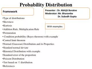
Framework. Presenter : Dr. Abhijit Boratne Moderator: Mr. Bharambe Dr. Subodh Gupta. Probability Distribution. With examples. Type of distributions Skewness Kurtosis Addition Rule, Multiplication Rule Permutation Condition probability (Bayes theorem) with example

Probability Distribution
E N D
Presentation Transcript
Framework Presenter : Dr. Abhijit Boratne Moderator: Mr. Bharambe Dr. Subodh Gupta Probability Distribution With examples Type of distributions Skewness Kurtosis Addition Rule, Multiplication Rule Permutation Condition probability (Bayes theorem) with example Central limit theorem Normal (Gaussian) Distribution and its Properties Standard normal deviate Binomial Distribution with example Standard error of the proportion Poisson Distribution Test based on ‘t’ disrtibution References
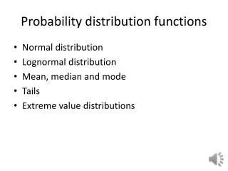
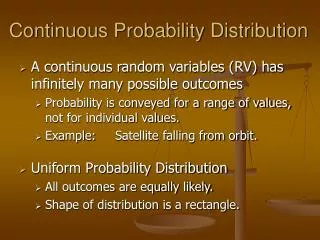
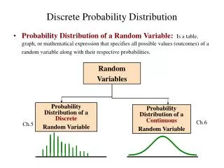
Types of Distribution • Continuous Distribution • Normal Distribution • Geometric distribution • Exponential distribution • Uniform distribution • Discrete distribution • Binomial Distribution • Poisson Distribution
Skewness • Skewness means lack of symmetry. • It indicates whether the curve is turned more to one side than to other, i.e. the curve has a longer tail on one side. • It can be positive or negative. • If curve is more elongated to the right side , i.e. the mean of the distribution is more than the mode. • Skewness is said to be negative if curve is more elongated to the left side i.e. the mean of the distribution is smaller than mode. Karl Pearson’s coefficient of skewness = Mean-Mode/SD Coefficient of skewness is pure number and it is zero for symmetrical distribution.
Kurtosis • The relative flatness or peakedness of the frequency curve. • Formula, ß2=μ4/μ22 • μ4= 1/n∑ifi(xi-x)4 in case of frequency distribution =1/n ∑i (xi-x)4 in case of individual values μ2= 1/n∑ifi(xi-x)2 in case of frequency distribution = 1/n ∑i (xi-x)2 in case of individual values
Probability • It is the chance factor for an event to occur or not to occur. • Probability is a mathematical quantity. • It can be presented as: P= P(A)=A/N=No. of favorable events/ No. of total events • If probability of an event happening is p and not happening is denoted by q, then q=1-p OR p+q=1 • Probability is usually denoted by “P”. Also, probability of event A is denoted by P(A), so probability of non occurrence of A is denoted by Q(A) Q(A)=no of non favorable events/N Total no of events-no of favorable events/total no of event =N-A/N =1-A/N =1-P
Addition Rule: Law of Additivity • Addition rule applies to a situation where we want probability for ‘one of this OR one of that’. • Turning up a one or two on a dice gives probability P(A or B)= P(A U B)= P(A) + P(B) =1/6 +1/6= 1/3 (here events are mutually exclusive) b) (When events are not mutually exclusive) we have to deduct the overlapping probability (i.e. probability of an ace heart) probability of an Ace heart P= Probability of heart +probability of Ace-Probability of Heart and Ace 13/52 + 4/52 - 1/52 P=16/52 OR=U called as union
Multiplication Rule • The probability that an event will occur jointly is the product of the probabilities of each event. • If A and B are independent events, then probability that A and B will occur is, P(AB)=P(A∩B)=P(A) P (B) Probability of head when coin tossed twice = 1/2 * 1/2=1/4 (here each toss is independent) • 3 out of 10 traffic accidents are fatal, probability of death by one accident is =3/10=0.3 • Probability of death by two successive accident is =3/10 * 3/10 =9/100 And = ∩ called as intersection
Permutation • Permutation means “order of occurrence” Examples: 1. two alphabets (a and b) It can be arrange as ab or ba 2. a,b,c can be arranged in following orders: a,b,c, a,c,b, b,a,c, b,c,a c,a,b c,b,a 3. Similarly 1,2,3 can be written as 1,2,3 1,3,2 2,1,3 2,3,1 3,1,2 3,2,1 Each of these is a different permutation
Condition probability (Bayes theorem) • In probability theory, Bayes' theorem relates the conditional and marginal probabilities of two random events. It is often used to compute posterior probabilities given observations. • Statement of Bayes' theorem • Bayes' theorem relates the conditional and marginal probabilities of events A and B, where B has a non-vanishing probability: P(A/B)=P(B/A) P(A)/P(B) P(A) is the prior probability or marginal probability of A. It is "prior" in the sense that it does not take into account any information about B. P(A|B) is the conditional probability of A, given B. It is also called the posterior probability because it is derived from or depends upon the specified value of B. P(B|A) is the conditional probability of B given A. P(B) is the prior or marginal probability of B, and acts as a normalizing constant.
Derivation from conditional probabilities • To derive the theorem, we start from the definition of conditional probability. The probability of event A given event B is P(A/B)=P(A∩B)/P(B) • Equivalently, the probability of event B given event A is P(B/A)= P(A∩B)/P(A) • Rearranging and combining these two equations, we find P(A/B) P(B)=P(A∩B)=P(B/A) P(A) • This lemma is sometimes called the product rule for probabilities. Dividing both sides by P(B), providing that it is non-zero, we obtain Bayes' theorem: • P(A/B)= P(A∩B)/P(B)= P(B/A) P(A)/P(B)
Example: Suppose there are two bowls full of cookies. Bowl #1 has 10 chocolate chip cookies and 30 plain cookies, while bowl #2 has 20 of each. Fred picks a bowl at random, and then picks a cookie at random. We may assume there is no reason to believe Fred treats one bowl differently from another, likewise for the cookies. The cookie turns out to be a plain one. How probable is it that Fred picked it out of bowl #1? • Intuitively, this should be greater than half since bowl #1 contains the same number of cookies as bowl #2, yet it has more plain. • We can clarify the situation by rephrasing the question to "what’s the probability that Fred picked bowl #1, given that he has a plain cookie?” The event A is that Fred picked bowl #1, and the event B is that Fred picked a plain cookie. To compute P(A|B), we first need to know:
P(A), or the probability that Fred picked bowl #1 regardless of any other information. Since Fred is treating both bowls equally, it is 0.5. • P(B), or the probability of getting a plain cookie regardless of any other information. Since there are 80 total cookies, and 50 of them are plain, the probability of selecting a plain cookie is 50/80 = 0.625. • P(B|A), or the probability of getting a plain cookie given Fred picked bowl #1. Since there are 40 cookies in bowl #1 and 30 of them are plain, the probability is 30/40 = 0.75. • Given all this information, we can compute the probability of Fred having selected bowl #1 given that he got a plain cookie by substitution: P(A/B)= P(B/A) P(A)/P(B)=0.75*0.5/0.625=0.6 As we expected, it is more than half.
Central limit theorem • If X is the mean of a random sample X1, X2, … Xn from a distribution with • mean μ and finite variance σ2 > 0, then the distribution of • Z=X-μ/σ√ n=Σnx=i Xi-nu/ σ√ n approaches a distribution that is N(0,1) as n becomes large.5 • In other words, when sampling from such a distribution (normal or otherwise), as the sample size increases, the distribution of X gets closer to a normal distribution. When sampling from a normal distribution, the distribution of X will, necessarily, be normal. • But , none of this implies that when larger samples are taken from a nonnormal distribution the underlying distribution itself becomes normally distributed. Rather, one would witness a clearer picture of the actual (nonnormal) distribution itself. The CLT discussed above is involved with assessing the distribution of X , not X—the individual values themselves.
Normal (Gaussian) Distribution 68.27 % 95.45 % 99.73 %
Properties of Normal Distribution • Distribution is continuous symmetrical curve where both tails extending to infinity. • All the measures of central tendency (mean, median and mode) are equal. • Mean determine the centre of the curve. • Skewness is equal to zero. • If the curve is transferred to a graph, the frequency curve will be bell shaped. • In any observation, the more the biological observation, the more it tends to follow the normal distribution and has a symmetrical dimension.
Properties of Normal Distribution cont… • The spread or variation around mean is represented by б. • Larger the SD greater is the spread of values. • Between μ ±1 б area is 68%, between μ ±2 б area is 95%, and between μ ±3 б area is 99%, of the total area of the curve.
Confidence Interval • As we can not draw large number of samples covering entire population in order to find population mean(μ), so we set up certain limits on the both sides of the population mean on the basis of the facts that means X of samples of size 30 or more are normally distributed around population mean μ. • This limits are called as confidence limit and the range bet the two is called as confidence interval. • As per the normal distribution of samples, we say with confidence that 95% of the sample means will lie within the confidence limits of μ-1.96SE(X) and 1+1.96SE(X) • The probability of occurrence of sample value out side this will be only 5% i.e. 0.05 , means 5/100=1/20 i.e. one in 20 times. • A CI can be used to describe how reliable survey results are.
Standard normal deviate • In any normal curve, it is possible to relate the distance between any observed value (x) and the mean of the curve (μ) as x- μ distance which is called as standard normal deviate or relative normal deviate. Z= x- μ / б e.g. population sample Mean ht=9” observed ht=18” SD of the normal curve=5” So, Z= x- μ / б , Z=18-9/5 Z=9/5=1.8 This means that x can be located at 2 SD distance from the centre of the curve.
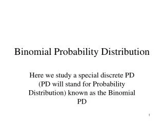
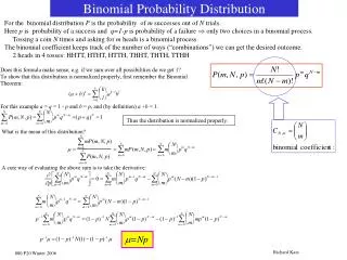
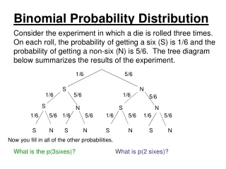
Binomial Distribution • Developed by Prof. James Bernoulli • The binomial distribution describes the distribution of discrete events or qualitative data. A random variables follow a binomial distribution when each trial has exactly two outcomes. • if p is the probability of occurrence in one trial, q is the probability of non occurrence in same trial (q=1-p ) and n is the number of trials, the probability distribution of outcomes is described by the terms of the expansion of the binomial distribution; (p+q)n, the probability of an event to occur is 1, thus p+q=1, q=1-p , So the expression will be (p+q)n =pn+nc1pn-1q+nc2pn-2q2+…+ncrpn-rqr+…+qn Where ncr=n!/r!(n-r)! When p is very much larger or very much smaller than q, the curve of distribution is quite asymmetrical when “n” is small. In cases like these, Poisson distribution is utilized.
Example: what are the chances of getting any combination, i.e. 2 boys, 1 girl or 1 boy and 2 girls or three boys or three girls when number of pregnancy is 3? Probability of getting boy or girl if found to be 0.5. • Expression, (p+q)n =(p+q)3 • (p+q)n=(p+q)3 =p3+3p2q+3pq2+q3 • P=0.5, q=1-o.5=0.5, n=3 • All children to be male:p3=(0.5)3=0.125 or 12.5% • All children to be female:q3=(0.5)3=0.125 or 12.5% • Two children male, third female:3p2q=3(0.5)2(0.5)=0.375 or 37.5% • Two children female, one male:3pq2=3(0.5)2(0.5)=0.375 or 37.5%
Standard error of the proportion • Z =x- μ / б in normal distribution. • In binomial distribution, use √pq /n • In a nature proportion of male is 51%. Supposed in sample (n=100) it is 39%. What inference do we draw? • SE= √pq /n = √51*49/100=4.99 • The value range we get is 51+ 1(4.99)=56 51-1(4.99)=46, so it can vary from 46 to 56 percent. In above sample is it 39, which is outside the limit. So it is not likely by chance. Z=51-39/4.99=2.40 Since relative deviate exceed 2.0, the deviation is significant.
Poisson Distribution • It is a discrete distribution • Its occurrence is towards impossible (where p is too small) • Used in social and physical sciences. • It was derived by S.D. Poisson(1781-1840) in 1837. • So, this is a limiting distribution of binomial distribution when the number of trials “n” is very large and the probability “p” is too small; the np is fixed number which is called as Poisson distribution • Formula, P=(X=x) e-λ λ x/x! Where x=a count 0,1,2,3,4,5,etc e=base of natural log=2.7181 λ=mean=variance μ=б2
Simplified version Px=em mx/x! Where e=constant m= μ x=distribution x!=factorial Under the following condition, we observe that distribution becoming Poisson: • Value of p or q becomes indefinitely small • Number of observation becomes (n) very large • The product of (n) and (p) which is np=mean number of event is always finite
Test based on ‘t’ Distribution • It is discovered by WA Gosset who published this under the pen name “Student” • In case of observations that are naturally paired the “t” test is applied to the mean of the differences between these pairs. This is to visualized whether such a mean is significantly less, greater or zero. • The general procedure followed: • Calculation of pooled SD • Use of pooled SD to calculate SE • Ratio of observed difference to SE • “t” table helps us in drawing inference In “t” distribution the DF used is equal to n-1 or less than the size of sample. When “t” test involves the difference between two means the DF is n1+n2-2
Formula t =x-μ/S/√n Where x=mean of the sample μ= mean of the population S= SD of the sample mean √n= number of observations Common applications: • To test the difference bet sample mean and population mean t =x-μ/S/√n where S=√∑(x-x)2/n-1 DF=n-1 2. To test for the difference bet two sample means t= x1-x2/S √1/n1+1/n2 Where x1and x2 are means of two sample S=pooled SD which is found out by S= √n1S21+n2S22/n1+n2-2 S21=variance of sample I= √∑(x1-x)2/n1-1 S22=variance of sample II= √∑(x2-x)2/n2-1 Where n1 n2 are sample sizes. DF will be n1+n2-2
3. To test for paired observations Take the difference bet data of pair directly. If there is no difference, it is zero, if it is more then it is positive and if it is less then it is negative. t= d/ S/√n where d=avg of the differences bet paired observation S= √∑(d1-d)2/n-1 • Diff under each category pair is noted reference made above • Mean of these diff is found out d • NH is set d=0 • Sample SD is found where n is number of pair of observation • Applying t test formula • Statistical inference, with Df=n-1 4. To test for the correlation coefficient t= r √n-2/√1-r2 where , r=correlation coefficient DF=n-2
References • Hill AB, Hill ID. Bradford Hill’s principles of medical statistics.First Indian edition.New Delhi:B.I.Publication Pvt Ltd; 1993.p.129. • Lwanga SK, Tye CY, Ayeni O. Teaching Health Statistics.WHO.First edition. Jeneva: WHO library; 1999.p58-65. • Armitage P, Berry G. Statistical Methods in Medical Research. Third edition. Cambridge: Oxford; 1994.p.48-52 • Mahajan BK. Methods in Biostatistics.6th Edition. Reprint . New Delhi: Jaypee Brothers;2005. p.117-120. • Rao KV. Biostatistics, A manual of statistical methods for use in health, nutrition and anthropology. Second edition. New Delhi:Jaypee Brothers;2007.p-63-89. • Prabhakara GN. Biostatistics. First edition. New Delhi:Jaypee Brothers;2006. p.89-94, 129-135.