Binomial Probability Distribution
Binomial Probability Distribution. Permutations. Number of possible arrangements. Combinations. Number of sets or groups. Binomial Theorem. Binomial Distribution.

Binomial Probability Distribution
E N D
Presentation Transcript
Binomial Probability Distribution
Permutations Number of possible arrangements
Combinations Number of sets or groups
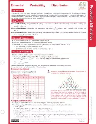
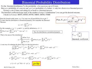
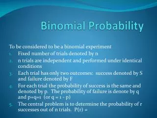
Binomial Distribution The binomial distribution is the probability distribution that results from sampling a binomial population. Binomial samples have the following properties: 1. Fixed number of trials, represented as n. 2. Each trial has two possible outcomes, a “success” and a “failure”. 3. P(success)=p (and thus: P(failure)=1–p), for all trials. 4. The trials are independent, which means that the outcome of one trial does not affect the outcomes of any other trials. May be population is large enough that sampling without replacement does not change values.
Success and Failure… …are just labels for a binomial experiment, there is no value judgment implied. For example a coin flip will result in either heads or tails. If we define “heads” as success then necessarily “tails” is considered a failure (in as much as we attempting to have the coin lands heads up). Other binomial experiment notions: An election candidate wins or loses An employee is male or female
Example Pat Statsdud is a (not good) student taking a statistics course. Pat’s exam strategy is to rely on luck for the next quiz. The quiz consists of 10 multiple-choice questions. Each question has five possible answers, only one of which is correct. Pat plans to guess the answer to each question. What is the probability that Pat gets no answers correct? What is the probability that Pat gets two answers correct?
Pat Statsdud… Algebraically then: n=10, and P(success)= 1/5 = .20 • Pat plans to guess the answer to each question. • Is this a binomial experiment? Check the conditions: • There is a fixed finite number of trials (n=10). • An answer can be either correct or incorrect. • The probability of a correct answer (P(success)=.20) does not change from question to question. • Each answer is independent of the others.
Pat Statsdud… n=10, and P(success) = .20 a. What is the probability that Pat gets no answers correct? i.e. # success, x, = 0; hence we want to know P(x=0) Pat has about an 11% chance of getting no answers correct using the guessing strategy.
Pat Statsdud… n=10, and P(success) = .20 b. What is the probability that Pat gets two answers correct? I.e. # success, x, = 2; hence we want to know P(x=2) Pat has about a 30% chance of getting exactly two answers correct using the guessing strategy.
Binomial Probability Distribution The binomial distribution with ntrials and success probabilityphas: • Mean = • Variance = • Standard deviation =
Cumulative Probability… Thus far, we have been using the binomial probability distribution to find probabilities for individual values of x. To answer the question: (Example 10) “Find the probability that Pat fails the quiz” requires a cumulative probability, that is, P(X ≤ x) If a grade on the quiz is less than 50% (i.e. 5 questions out of 10), that’s considered a failed quiz. Thus, we want to know what is: P(X ≤ 4) to answer
Pat Statsdud P(X ≤ 4) = P(0) + P(1) + P(2) + P(3) + P(4) We already know P(0) = .1074 and P(2) = .3020. Using the binomial formula to calculate the others: P(1) = .2684 , P(3) = .2013, and P(4) = .0881 We have P(X ≤ 4) = .1074 + .2684 + … + .0881 = .9672 Thus, its about 97% probable that Pat will fail the test using the luck strategy and guessing at answers…
Pat Statsdud Has Been Cloned Suppose that a professor has a class full of students like Pat. What is the mean? What is the standard deviation? The mean = μ = np = 10(0.2) = 2 The standard deviation is σ= √np( 1 – p ) = √10( .2)( 1 - .2) = 1.26
Lock Section 6.1 Sampling Distribution of the Sample Proportion
Binomial Population Two Choices: Success Failure Fixed Probability Independence
Properties of p-hat • When sample sizes are fairly large, the shape of the p-hat distribution will be normal. • The mean of the distribution is the value of the population parameter p. • The standard deviation of this distribution is the square root of p(1-p)/n.
Sampling Distribution of p-hat For the sampling distribution to be normal, you must have:
Calculate Probabilities • Because the shape of the distribution is normal, we can standardize the variable p-hat to a Z standard normal distribution. Use Z-transform:
Lock Section 6.2 Confidence Intervals for Population Proportions AP Statistics
Confidence Intervals Confidence Intervals Population Mean Population Proportion σKnown σUnknown AP Statistics
Confidence Intervals for the Population Proportion, p • Recall that the distribution of the sample proportion is approximately normal if the sample size is large, with standard deviation • We will estimate this with sample data: AP Statistics
How Big???? • Rule of Thumb 1: Formula for standard deviation of p-hat only when the population, N, is at least 10 times the sample size: N ≥ 10 n • Rule of Thumb 2: The sampling distribution of p-hat is approximately Normal when • np ≥ 10 and n(1-p) ≥ 10
Confidence interval endpoints • Upper and lower confidence limits for the population proportion are calculated with the formula • where • z is the standard normal value for the level of confidence desired • p is the sample proportion • n is the sample size AP Statistics
Example • A random sample of 100 people shows that 25 are left-handed. • Form a 95% confidence interval for the true proportion of left-handers AP Statistics
Example (continued) • A random sample of 100 people shows that 25 are left-handed. Form a 95% confidence interval for the true proportion of left-handers. 1. 2. 3. AP Statistics
Interpretation • We are 95% confident that the true percentage of left-handers in the population is between 16.51% and 33.49%. • Although this range may or may not contain the true proportion, 95% of intervals formed from samples of size 100 in this manner will contain the true proportion. AP Statistics
Changing the sample size • Increases in the sample size reduce the width of the confidence interval. Example: • If the sample size in the above example is doubled to 200, and if 50 are left-handed in the sample, then the interval is still centered at .25, but the width shrinks to .19 …… .31 AP Statistics
Example 2 • A random sample of 400 graduates showed 32 went to grad school. Set up a 95% confidence interval estimate for p.
Example 2 • A random sample of 400 graduates showed 32 went to grad school. Set up a 95% confidence interval estimate for p.
Thinking Challenge • You’re a production manager for a newspaper. You want to find the % defective. Of 200 newspapers, 35 had defects. What is the 90% confidence interval estimate of the population proportion defective?
Required Sample Size Define the margin of error: Solve for n: p can be estimated with a pilot sample, if necessary (or conservatively use p = .50) AP Statistics
What sample size...? • How large a sample would be necessary to estimate the true proportion defective in a large population within 3%,with 95% confidence? (Assume a pilot sample yields p-hat = .12) AP Statistics
What sample size...? (continued) Solution: For 95% confidence, use Z = 1.96 E = .03 P-hat = .12, so use this to estimate p So use n = 451 AP Statistics
Lock Section 6.3 Hypothesis Tests For Single Proportions
Test of Proportions • Old drug cures 80 percent of the time. New drug for heartworm disease in dogs cures 90 percent of n=1000 dogs, so p-hat=.9. • What is the probability that this results occurred by random chance?