Understanding Probability Distributions in Statistics
Learn about various probability distributions, including discrete, binomial, normal, and more. Explore calculating mean, variance, and applying distributions in real-world scenarios. Practice problems included.


Understanding Probability Distributions in Statistics
E N D
Presentation Transcript
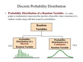
Probability Distributions • A probability distribution is a listing of all the outcomes of an experiment and the probability associated with each outcome. • Characteristics of a Probability Distribution • The probability of an outcome must always be between 0 and 1. • The sum of all mutually exclusive outcomes is always 1.
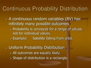
Random Variables • A random variable is a numerical value determined by the outcome of an experiment • A discrete random variable is a variable that can assume only certain clearly separated values resulting from a count of some item of interest. • A continuous random variable is a variable that can assume one of an infinitely large number of values resulting from measuring something
Types of Probability Distributions • Discrete Probability Distributions • Binomial Probability Distributions • Hypergeometric Probability Distributions • Poisson Probability Distributions • Continuous Probability Distributions • Normal Probability Distributions
The Mean of a Discrete Probability Distribution • Reports the central location of the data. • The Mean is the long-run average value of the random variable. • The Mean is also referred to as its expected value, E(x), in a probability distribution. • The Mean is a weighted average. • The mean is computed by the formula:
The Variance & Standard Distribution of a Discrete Probability Distribution • The variance, , measures the amount of spread (variation) of a distribution. • The standard deviation, , is obtained by taking the square root of variance. • The variance of a discrete probability distribution is computed from the formula
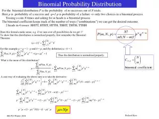
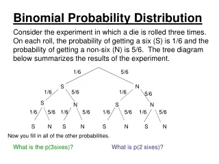
Binomial Probability Distribution • The Binomial Distribution has the following characteristics: • An outcome of an experiment is classified into one of two mutually exclusive categories : success or failure. • The probability of success stays the same for each trial. • The distribution results from a count of the number of successes in a fixed number of trials. • The trials are independent.
cont.. • The formula for the binomial probability distribution is: • n be the number of trials • x be the number of observed successes • be the probability of success on each trial
Contoh: • Sebuah ujian berisikan empat pertanyaan benar/salah dan seorang mahasiswa tidak mempunyai sedikit pun topik ujian tersebut. • Jadi peluang mahasiswa menebak jawaban yang tepat pada pertanyaan pertama = 0.5 dan probabilitas menebak jawaban berikutnya secara tepat 0.5 • Berapakah : a. Mendapatkan tidak satupun dari empat pertanyaan yang tepat b. Mendapatkan tepat satu dari empat pertanyaan yang tepat
a. Mendapatkan tidak satupun dari empat pertanyaan yang tepat b. Mendapatkan tepat satu dari empat pertanyaan yang tepat
Binomial Probability Distribution • The mean is given by: • The variance is given by: • The binomial distribution of probabilities will become more and more skewed to the right as the probability of success become smaller
Contoh • Probabilitas kerusakan pada barang yang diproduksi Perusahaan “X” adalah 10%. Jika diambil 6 sampel random, maka : • Buatlah distribusi probabilitas • Hitung rata-rata dan standar deviasi probabilitas tersebut
Soal • Berdasarkan data sebelumnya, probabilitas mahasiswa lulus Mata Kuliah Statistik adalah 70%. Jika diambil sampel random 10 mahasiswa, hitung probabilitas • 6 mahasiswa lulus • 3 mahasiswa tidak lulus • Kurang dari 9 mahasiswa lulus • Paling banyak 2 mahasiswa tidak lulus
Hypergeometric Probability Distribution • The Hypergeometric Distribution has the following characteristics: • There are two mutually exclusive categories : success or failure. • The probability of success is not the same for each trial. • The distribution results from a count of the number of successes in a fixed number of trials.
cont.. • the sample is selected from a finite population (the number of population is known and relatively small) without replacement • the size of the sample n is greater than 5% of the size of the population N. • Note : Rule of Thumb If the selected items are not returned to the population and the sample size is less than 5 percent of the population (n < 0,05N), the binomial distribution can be used to approximate the hypergeometric distribution.
Hypergeometric Probability Distribution • Formula : • N : the size of the population • S : the number of successes in the population • x : the number of successes of interest • n : the sample size • C : a combination.
Contoh • Perusahaan “X” mempunyai 50 karyawan, 40 diantaranya bergabung dalam Serikat Kerja. Jika diambil 5 sampel random, maka : • Berapa probabilitas 4 karyawan bergabung dalam Serikat Kerja • Buat distribusi probabilitas
Poisson Probability Distribution • It describes the number of times some events occur during a specified interval (the interval may be time, distance, area, or volume) • The probability of a “success” is proportional to the length of the interval (the longer the interval, the larger the probability) • The intervals are independent • The limiting form of the binomial distribution where the probability of success is very small and n is large (“The law of improbable events”)
cont.. • The Poisson distribution can be described mathematically using the formula: • : the arithmetic mean number of occurrences in a particular interval of time • e : the constant 2.71828 (base on the Naperian logarithmic system) • x : the number of occurrences.
Contoh • 2% mahasiswa Fakultas Ekonomi tidak lulus dalam ujian Mata Kuliah Pengantar Bisnis. Jika 1000 mahasiswa ikut ujian tersebut, berapakah probabilitas : • 3 mahasiswa tidak lulus • Minimal 2 mahasiswa tidak lulus
Characteristics of a Normal Probability Distribution • The normal curve is bell-shaped and has a single peak at the exact center of the distribution.The arithmetic mean, median, and mode of the distribution are equal and located at the peak. • The normal probability distribution is symmetrical about its mean • The normal probability distribution is asymptotic (the curve gets closer and closer to the x-axis but never actually touches it). • It is completely described by Mean & Standard Deviation • There is a family of normal distribution. Each time The Mean & Standard Deviation change, a a new distribution is created
r a l i t r b u i o n : m = 0 , s2 = 1 0 . 4 0 . 3 0 . 2 x ( f 0 . 1 . 0 - 5 x Characteristics of a Normal Distribution Normal curve is symmetrical Theoretically, curve extends to infinity a Mean, median, and mode are equal
The Standard Normal Probability Distribution • A normal distribution with a mean of 0 and a standard deviation of 1 is called the standard normal distribution. • Z value: The distance between a selected value, designated X, and the population mean ( ), divided by the population standard deviation ( ) • Z value = Z score = Z statistic = the standard normal deviate = normal deviate
Areas Under the Normal Curve • About 68 percent of the area under the normal curve is within one standard deviation of the mean. • About 95 percent is within two standard deviations of the mean. • 99.74 percent is within three standard deviations of the mean.
m-2s m-1s m m+1s m+2s m+ 3s m-3s
Contoh Penerapan Distribusi Normal Baku • Diketahui: penghasilan mingguan manajer madya secara normal dengan rata-rata hitung 1000 dan standar deviasi 100. • Berapakah nilai daerah di bawah kurva normal terletak di antara 1000 dan 1100? Lihat Tabel Z (lampiran D) nilainya 0,3413
Gambar: 0,3413 1100 1000
Soal • Hasil survey thd 300 penduduk ttg pendapatan per bulan : rata-rata $100 dengan simpangan baku $15 Jika diasumsikan data pendapatan mengikuti distribusi normal, maka hitung : • Berapa persen penduduk yang berpendapatan $75-$130 • Berapa persen penduduk yang berpendapatan $110-$115 • Berapa persen penduduk yang berpendapatan kurang dari $90 • Jika Pemerintah mengenakan pajak terhadap 10% penduduk terkaya, maka berapa batas pendapatan terendah kena pajak • Jika Pemerintah memberikan subsidi terhadap 20% penduduk termiskin, maka berapakah batas pendapatan tertinggi yang memenuhi persyaratan
Central Limit Theorem • If all sample of particular size are selected from any population, the sampling distribution of the sample mean is approximately a normal distribution. The approximation improves with larger samples. • If a the population follows a normal probability distribution, then for any sample size the sampling distribution on the sample mean will also normal. • As we increase the size of sample, the spread of the sample mean becomes smaller • Most statisticians consider a sample of 30 of more to be large enough for the central limit theorem to be employed
The Normal Approximation to the Binomial • Using the normal distribution (a continuous distribution) as a substitute for a binomial distribution (a discrete distribution) for large values of n seems reasonable because as n increases, a binomial distribution gets closer and closer to a normal distribution. • The normal probability distribution is generally deemed a good approximation to the binomial probability distribution when n and n(1- ) are both greater than 5.
Continuity Correction Factor • The value 0.5 subtracted or added, depending on the problem, to a selected value when a binomial probability distribution (a discrete probability distribution) is being approximated by a continuous probability distribution (the normal distribution). • For the P at least X occur, use the area above (X – 0,5) • For the P that more than X occur, use the area above (X + 0,5) • For the P that X or fewer occur, use the area below (X + 0,5) • For the P that fewer than X occur, use the area below (X – 0,5)
Soal • BLM melakukan polling dengan menyebarkan 60 kuesioner. Probabilitas kembalinya kuisioner adalah 80%. Hitung probabilitas : • 50 kuisioner kembali • Antara 45-55 kuesioner kembali • Kurang dari 55 kuesioner kembali • 20 atau lebih kuesioner kembali