Plotting Continuous Functions Using Linspace and Array Operations
This guide covers the techniques for plotting continuous functions, particularly utilizing the `linspace` function and various array operations. It illustrates how to generate plots of functions like `y = sin(x)` and `y = exp(x)` over specified ranges, creating smooth curves by using an adequate number of points. The document demonstrates examples involving basic arithmetic operations on arrays, ensuring the application of vectorized operations for efficiency. Additionally, it addresses common plotting scenarios including negation, scaling, and division of arrays.

Plotting Continuous Functions Using Linspace and Array Operations
E N D
Presentation Transcript
10. Plotting Continuous Functions Linspace Array Operations
Table Plot x sin(x) 0.00 0.0 1.57 1.0 3.14 0.0 4.71 -1.0 6.28 0.0 Plot based on 5 points
Table Plot x sin(x) 0.000 0.000 0.784 0.707 1.571 1.000 2.357 0.707 3.142 0.000 3.927 -0.707 4.712 -1.000 5.498 -0.707 6.283 0.000 Plot based on 9 points
Table Plot Plot based on 200 points—looks smooth
Generating Tables and Plots x sin(x) 0.000 0.000 0.784 0.707 1.571 1.000 2.357 0.707 3.142 0.000 3.927 -0.707 4.712 -1.000 5.498 -0.707 6.283 0.000 x = linspace(0,2*pi,9); y = sin(x); plot(x,y)
linspace x = linspace(1,3,5) x : 1.0 1.5 2.0 2.5 3.0 “x is a table of values” “x is an array” “x is a vector”
linspace x = linspace(0,1,101) … x : 0.00 0.01 0.02 0.99 1.00
Linspace Syntax linspace( , , ) Number of Points Left Endpoint Right Endpoint
Built-In Functions Accept Arrays 0.00 1.57 3.14 4.71 6.28 sin x sin(x) 0.00 0.0 1.57 1.0 3.14 0.0 4.71 -1.0 6.28 0.0 And…
Return Array of Function-evals sin 0.00 1.00 0.00 -1.00 0.00 x sin(x) 0.00 0.0 1.57 1.0 3.14 0.0 4.71 -1.0 6.28 0.0
Examples x = linspace(0,1,200); y = exp(x); plot(x,y) x = linspace(1,10,200); y = log(x); plot(x,y)
Can We Plot This? -2 <= x <= 3
Can We Plot This? -2 <= x <= 3 Yes! x = linspace(-2,3,200); y = sin(5*x).*exp(-x/2)./(1 + x.^2) plot(x,y) Array operations
Must LearnHow to Operate on Arrays Look at four simpler plotting challenges.
Scale (*) a: -5 8 10 c = s*a s: 2 20 16 -10 c:
Addition a: -5 8 10 c = a + b b: 2 1 4 12 12 -4 c:
Subtraction a: -5 8 10 c = a - b b: 2 1 4 8 4 -6 c:
E.g.1 Sol’n x = linspace(0,4*pi,200); y1 = sin(x); y2 = cos(3*x); y3 = sin(20*x); y = 2*y1 - y2 + .1*y3; plot(x,y)
Exponentiation a: -5 8 10 c = a.^s s: 2 .^ 100 64 25 c:
Shift a: -5 8 10 c = a + s s: 2 12 10 -3 c:
Reciprocation a: -5 8 10 c = 1./a .1 .125 -.2 c:
E.g.2 Sol’n x = linspace(-5,5,200); y = 5./(1+ x.^2); plot(x,y)
Negation a: -5 8 10 c = -a -10 -8 5 c:
Scale (/) a: -5 8 10 c = a/s s: 2 5 4 -2.5 c:
Multiplication a: -5 8 10 c = a .* b b: 2 1 4 .* 20 32 -5 c:
E.g.3 Sol’n x = linspace(0,3,200); y = exp(-x/2).*sin(10*x); plot(x,y)
Division a: -5 8 10 c = a ./ b b: 2 1 4 ./ 5 2 -5 c:
E.g.4 Sol’n x = linspace(-2*pi,2*pi,200); y = (.2*x.^3 - x)./(1.1 + cos(x)); plot(x,y)
Question Time How many errors in the following statement given that x = linspace(0,1,100): Y = (3*x .+ 1)/(1 + x^2) A. 0 B. 1 C. 2 D. 3 E. 4
Question Time How many errors in the following statement given that x = linspace(0,1,100): Y = (3*x .+ 1)/(1 + x^2) Y = (3*x + 1) ./ (1 + x.^2) A. 0 B. 1 C. 2 D. 3 E. 4
Question Time Does this assign to y the values sin(0o), sin(1o),…,sin(90o)? x = linspace(0,pi/2,90); y = sin(x); A. Yes B. No
Question Time Does this assign to y the values sin(0o), sin(1o),…,sin(90o)? %x = linspace(0,pi/2,90); x = linspace(0,pi/2,91); y = sin(x); A. Yes B. No
Plotting an Ellipse Better:
Solution a = input(‘Major semiaxis:’); b = input(‘Minor semiaxis:’); t = linspace(0,2*pi,200); x = a*cos(t); y = b*sin(t); plot(x,y) axis equal off