CHAPTER 6 Statistical Inference & Hypothesis Testing

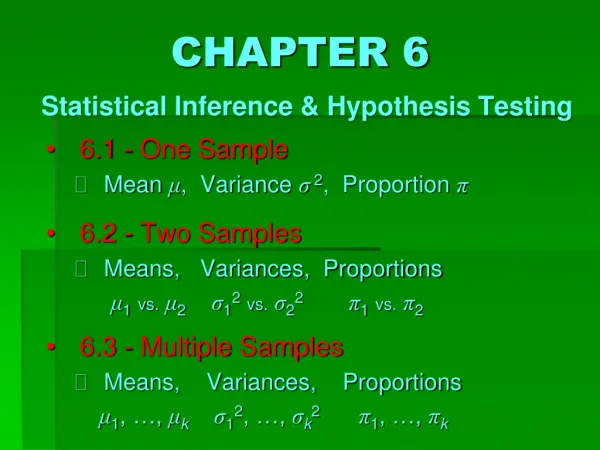
CHAPTER 6Statistical Inference & Hypothesis Testing 6.1 - One Sample Mean μ, Variance σ2, Proportion π 6.2 - Two Samples Means, Variances, Proportions μ1vs.μ2σ12vs.σ22π1vs.π2 6.3 - Multiple Samples Means, Variances, Proportions μ1, …, μkσ12, …,σk2π1, …, πk

Example: One Mean POPULATION “Random Variable” X = Age (years) Objective 1: “Parameter Estimation” Women in U.S. who have given birth Improve this point estimate of μ to an “interval estimate” of μ, via the… Present: Assume that X follows a “normal distribution” in the population, with std dev σ = 1.5 yrs, but unknown mean μ= ? That is, X~N(μ, 1.5). “Sampling Distribution of ” Estimate the parameter value μ. standard deviation σ= 1.5 This is referred to as a “point estimate” of μ from the sample. mean mean μ= ??? Random Sample size n = 400 FORMULA {x1, x2, x3, x4, … , x400}

Population Distribution of X If X ~ N(μ, σ), then… for any sample size n. “standard error” X = Age of women in U.S. who have given birth Sampling Distribution of standard deviation σ = 1.5 yrs X μ μ

Suppose is any random sample mean. | μ “standard error” To achieve Objective 1 — obtain an “interval estimate” of μ — we first ask the following general question: Sampling Distribution of Find a “margin of error” (d)so that there is a 95% probability that the interval contains μ. μ

d = (z.025)(s.e.) = (1.96)(.075 yrs) = 0.147 yrs | μ “standard error” Sampling Distribution of standard normal distribution N(0, 1) 0.95 0.025 0.025 Z μ +z.025 -z.025

d = (z.025)(s.e.) = (1.96)(.075 yrs) = 0.147 yrs IMPORTANT DEF’NS and FACTS d is called the “95% margin of error” and is equal to the product of the “.025 critical value” (i.e., z.025 = 1.96) times the “standard error” (i.e., ). | μ The “confidence level” is 95%. The “significance level” is 5%. For any random sample mean the “95% confidence interval” is It contains μwith probability 95%. standard normal distribution N(0, 1) In this example, the 95% CI is 0.95 For instance, if a particular sample yields the 95% CI is (25.6 – 0.147, 25.6 + 0.147) = (25.543, 25.747) yrs. It contains μwith 95% “confidence.” 0.025 0.025 Z +z.025 -z.025

d = (z.025)(s.e.) = (1.96)(.075 yrs) = 0.147 yrs IMPORTANT DEF’NS and FACTS d = (zα/2)(s.e.) “100(1 – α)% margin of error” d is called the “95% margin of error” and is equal to the product of the “.025 critical value” (i.e., z.025 = 1.96) times the “standard error” (i.e., ). “α/2 zα/2) | μ 1 – α The “confidence level” is 95%. 1 – α. The “significance level” is 5%. α. For any random sample mean the “95% confidence interval” is It contains μwith probability 95%. “100(1 – α)% “confidence interval” 1 – α. standard normal distribution N(0, 1) In this example, the 95% CI is 1 – α 0.95 For instance, if a particular sample yields the 95% CI is (25.6 – 0.147, 25.6 + 0.147) = (25.543, 25.747) yrs. It contains μwith 95% “confidence.” α/2 0.025 α/2 0.025 Z -zα/2 +zα/2 +z.025 -z.025

d = (zα/2)(s.e.) IMPORTANT DEF’NS and FACTS “100(1 – α)% margin of error” d is called the “95% margin of error” and is equal to the product of the “.025 critical value” (i.e., z.025 = 1.96) times the “standard error” (i.e., ). “α/2 zα/2) | μ 1 – α The “confidence level” is 95%. 1 – α. The “significance level” is 5%. α. For any random sample mean the “95% confidence interval” is It contains μwith probability 95%. “100(1 – α)% “confidence interval” 1 – α. standard normal distribution N(0, 1) What happens if we change α? Example:α = .01, 1 – α = .99 Example:α = .05, 1 – α = .95 Example:α = .10, 1 – α = .90 1 – α 0.95 -2.575 -1.96 -1.645 +1.645 +1.96 +2.575 | 0 α/2 0.025 α/2 0.025 Z Why not ask for α= 0, i.e., 1 – α= 1? -zα/2 +zα/2 +z.025 -z.025 Because then the critical values → ± ∞.

IMPORTANT DEF’NS and FACTS 95% margin of error (z.025)(s.e.) = (1.96)(.075 yrs) = 0.147 yrs ? μ | standard normal distribution N(0, 1) Z In this example, the 95% CI is 0.95 For instance, if a particular sample yields the 95% CI is (25.6 – 0.147, 25.6 + 0.147) = (25.543, 25.747) yrs. It contains μwith 95% “confidence.” 0.025 0.025 In principle, over the long run, the probability that a random interval contains μ will approach 95%. +1.96 -1.96 BUT…. … etc…

IMPORTANT DEF’NS and FACTS 95% margin of error (z.025)(s.e.) = (1.96)(.075 yrs) = 0.147 yrs μ | In practice, only a single, fixed interval is generated from a single random sample, so technically, “probability” does not apply. standard normal distribution N(0, 1) Z In this example, the 95% CI is 0.95 For instance, if a particular sample yields the 95% CI is (25.6 – 0.147, 25.6 + 0.147) = (25.543, 25.747) yrs. It contains μwith 95% “confidence.” 0.025 0.025 In principle, over the long run, the probability that a random interval contains μ will approach 95%. NOW, let us introduce and test a specific hypothesis… +1.96 -1.96 BUT….

Study Question: Has “age at first birth” of women in the U.S. changed over time? Statistical Inference and Hypothesis Testing POPULATION Women in U.S. who have given birth “Random Variable” X = Age at first birth “Null Hypothesis” Year 2010: Suppose we know that X follows a “normal distribution” (a.k.a. “bell curve”) in the population. Present: Is μ = 25.4 still true? H0: • public education, awareness programs • socioeconomic conditions, etc. Or, is the “alternative hypothesis” HA:μ ≠ 25.4 true? That is, X~N(25.4, 1.5). standard deviation σ = 1.5 i.e., either or ? (2-sided) μ < 25.4 μ > 25.4 μ > 25.4 μ < 25.4 Does the sample statistic tend to supportH0, or refuteH0 in favor of HA? mean mean μ = 25.4 Random Sample {x1, x2, x3, x4, … , x400} FORMULA

Objective 2: Hypothesis Testing… via Confidence Interval We have now seen: 95% CONFIDENCE INTERVAL FOR µ 25.543 25.747 “point estimate” for μ BASED ON OUR SAMPLE DATA, the true value of μ today is between 25.543 and 25.747, with 95% “confidence.” FORMAL CONCLUSIONS: The 95% confidence interval corresponding to our sample mean does not contain the “null value” of the population mean, μ = 25.4. Based on our sample data, we may reject the null hypothesis H0: μ = 25.4 in favor of the two-sided alternative hypothesis HA: μ ≠ 25.4, at the α = .05 significance level. INTERPRETATION:According to the results of this study, there exists a statistically significantdifference between the mean ages at first birth in 2010 (25.4 yrs) and today, at the 5% significance level. Moreover, the evidence from the sample data suggests that the population mean age today is older than in 2010, rather than younger. NOTE THAT THE CONFIDENCE INTERVAL ONLY DEPENDS ON THE SAMPLE, NOT A SPECIFIC NULL HYPOTHESIS!!!

Objective 2: Hypothesis Testing… via Confidence Interval What if…? We have now seen: 95% CONFIDENCE INTERVAL FOR µ 95% CONFIDENCE INTERVAL FOR µ 25.053 25.543 25.347 25.747 “point estimate” for μ “point estimate” for μ BASED ON OUR SAMPLE DATA, the true value of μ today is between 25.543 and 25.747, with 95% “confidence.” BASED ON OUR SAMPLE DATA, the true value of μ today is between 25.053 and 25.347, with 95% “confidence.” ? FORMAL CONCLUSIONS: The 95% confidence interval corresponding to our sample mean does not contain the “null value” of the population mean, μ = 25.4. Based on our sample data, we may reject the null hypothesis H0: μ = 25.4 in favor of the two-sided alternative hypothesis HA: μ ≠ 25.4, at the α = .05 significance level. INTERPRETATION:According to the results of this study, there exists a statistically significantdifference between the mean ages at first birth in 2010 (25.4 yrs) and today, at the 5% significance level. Moreover, the evidence from the sample data suggests that the population mean age today is older than in 2010, rather than younger. NOTE THAT THE CONFIDENCE INTERVAL ONLY DEPENDS ON THE SAMPLE, NOT A SPECIFIC NULL HYPOTHESIS!!! younger than in 2010, rather than older.

Objective 2: Hypothesis Testing… via Confidence Interval Objective 2: Hypothesis Testing… via Acceptance Region IF the null hypothesis H0: μ= 25.4 is indeed true, then… 95% margin of error (z.025)(s.e.) = (1.96)(.075 yrs) = 0.147 yrs | μ = 25.4 “standard error” “Null” Distribution of Sampling Distribution of … and out here… 0.95 …with 5% probability. … we would expect a random sample mean to lie in here, with 95% probability… 0.025 0.025 95% ACCEPTANCE REGION FOR H0 25.547 25.253 μ 25.4

Objective 2: Hypothesis Testing… via Acceptance Region Our data value lies in the 5% REJECTION REGION. We have now seen: 95% ACCEPTANCE REGION FOR H0 25.547 25.253 FORMAL CONCLUSIONS: The 95% acceptance region for the null hypothesis does not contain the sample mean of Based on our sample data, we may reject the null hypothesis H0: μ = 25.4 in favor of the two-sided alternative hypothesis HA: μ ≠ 25.4, at the α = .05 significance level. INTERPRETATION:According to the results of this study, there exists a statistically significantdifference between the mean ages at first birth in 2010 (25.4 yrs) and today, at the 5% significance level. Moreover, the evidence from the sample data suggests that the population mean age today is older than in 2010, rather than younger. NOTE THAT THE ACCEPTANCE REGION ONLY DEPENDS ON THE NULL HYPOTHESIS, NOT ON THE SAMPLE!!! IF H0 is true, then we would expect a random sample mean to lie between 25.253 and 25.547, with 95% probability.

Objective 2: Hypothesis Testing… via Acceptance Region Objective 2: Hypothesis Testing… via “p-value” - measures the strength of the rejection IF the null hypothesis H0: μ= 25.4 is indeed true, then… > 1.96 what is the probability of obtaining a random sample mean that is as, or more, extreme than the one actually obtained? i.e., 0.2 yrs OR MORE away from μ= 25.4, ON EITHER SIDE (since the alternative hypothesis is 2-sided)? 0.95 < .05 statistically significant 0.025 0.025 95% ACCEPTANCE REGION FOR H0 | μ = 25.4 0.00383 0.00383 25.253 25.547

Objective 2: Hypothesis Testing… via Acceptance Region Objective 2: Hypothesis Testing… via “p-value” - measures the strength of the rejection IF the null hypothesis H0: μ= 25.4 is indeed true, then… > 1.96 what is the probability of obtaining a random sample mean that is as, or more, extreme than the one actually obtained? i.e., 0.2 yrs OR MORE away from μ= 25.4, ON EITHER SIDE (since the alternative hypothesis is 2-sided)? 0.95 < .05 α statistically significant 0.025 0.025 1 – α 95% ACCEPTANCE REGION FOR H0 α/ 2 α/ 2 | μ = 25.4 0.00383 0.00383 100(1 – α)% ACCEPTANCE REGION FOR H0 25.253 25.547 -zα/2 +zα/2

... But interpret it correctly! If p-value < ,then reject H0; significance! p-value  = .05

~ Summary of Hypothesis Testing for One Mean ~ Assume the population random variable is normally distributed, i.e., XN(μ, σ). Test null hypothesis at significance level α. ALTERNATIVE HYPOTHESISHA: μμ0 NULL HYPOTHESISH0: μ = μ0(“null value”) i.e., either μ<μ0 or μ>μ0 (“two-sided”) zα/2 • CONFIDENCE INTERVAL • Compute the sample mean • Compute the 100(1 – α)% “margin of error” = (critical value)(standard error) • Then the 100(1 – α)% CI = • Formal Conclusion: • Reject null hypothesis at level α, Statistical significance! Otherwise, retain it. if CI does not contain μ0.

~ Summary of Hypothesis Testing for One Mean ~ Assume the population random variable is normally distributed, i.e., XN(μ, σ). Test null hypothesis at significance level α. ALTERNATIVE HYPOTHESISHA: μμ0 NULL HYPOTHESISH0: μ = μ0(“null value”) i.e., either μ<μ0 or μ>μ0 (“two-sided”) zα/2 • ACCEPTANCE REGION • Compute the sample mean • Compute the 100(1 – α)% “margin of error” = (critical value)(standard error) • Then the 100(1 – α)% AR = • Formal Conclusion: • Reject null hypothesis at level α, Statistical significance!Otherwise, retain it. if AR does not contain

~ Summary of Hypothesis Testing for One Mean ~ Assume the population random variable is normally distributed, i.e., XN(μ, σ). Test null hypothesis at significance level α. ALTERNATIVE HYPOTHESISHA: μμ0 NULL HYPOTHESISH0: μ = μ0(“null value”) i.e., either μ<μ0 or μ>μ0 (“two-sided”) • p-value • Compute the sample mean • Compute the z-score • If +, then the p-value = 2 P(Z≥ z-score ). • If –, then the p-value = 2 P(Z≤ z-score ). • Formal Conclusion: • Reject null hypothesis Statistical significance! Otherwise, retain it. • Remember: “The smaller the p-value, the stronger the rejection, and the more statistically significant the result.” Z ~ N(0, 1) z-score if p < α.

Objective 2: Hypothesis Testing… 1-sided tests The alternative hypothesis usually reflects the investigator’s belief! 2-sided test H0: μ = 25.4 HA: μ 25.4 p-value In this case,  = .05 is split evenly between the two tails, left and right. 1-sided tests “Right-tailed” H0: μ 25.4 HA: μ> 25.4 Here, all of  = .05 is in the right tail. < .05 The alternative hypothesis usually reflects the investigator’s belief! statistically significant 0.95 0.025 0.025 .00383 .00383 95% ACCEPTANCE REGION FOR H0 | μ = 25.4 25.253 25.547

Objective 2: Hypothesis Testing… 1-sided tests 2-sided test H0: μ = 25.4 HA: μ 25.4 p-value In this case,  = .05 is split evenly between the two tails, left and right. 1-sided tests “Right-tailed” H0: μ 25.4 HA: μ> 25.4 Here, all of  = .05 is in the right tail. < .05 statistically significant Use 1-sided tests sparingly! 0.95 0.05 0.025 0.025 .00383 .00383 95% ACCEPTANCE REGION FOR H0 95% ACCEPTANCE REGION FOR H0 | μ = 25.4 25.253 ? 25.547

Objective 2: Hypothesis Testing… 1-sided tests 2-sided test H0: μ = 25.4 HA: μ 25.4 p-value 25.2 25.2 In this case,  = .05 is split evenly between the two tails, left and right. 25.2 1-sided tests “Right-tailed” H0: μ 25.4 HA: μ> 25.4 Here, all of  = .05 is in the right tail. “Left-tailed” H0: μ 25.4 HA: μ < 25.4 Here, all of  = .05 is in the left tail. < .05 >> .05 The alternative hypothesis usually reflects the investigator’s belief! statistically significant strong support of null hypothesis 0.95 0.05 95% ACCEPTANCE REGION FOR H0 | μ = 25.4 ?

Calculate…fromH0 Test Statistic “z-score” = Calculate…fromH0 Test Statistic “z-score” = STATBOT 301 HA: μ < μ0 HA: μ < μ0 HA: μ > μ0 HA: μ > μ0 HA: μ ≠ μ0? HA: μ ≠ μ0? Subject: basic calculation of p-values for z-test 1 – table entry 1 – table entry table entry table entry sign of z-score? sign of z-score? – – + + 2 × table entry 2 × table entry 2 × (1 – table entry) 2 × (1 – table entry)

Example: One Mean POPULATION “Random Variable” X = Age (years) Objective 1: “Parameter Estimation” Women in U.S. who have given birth Improve this point estimate of μ to an “interval estimate” of μ, via the… Present: Assume that X follows a “normal distribution” in the population, with std dev σ = 1.5 yrs, but unknown mean μ= ? That is, XN(μ, 1.5). “Sampling Distribution of “ Estimate the parameter value μ. But how do we know that the variance is the same as in 2010? standard deviation σ = 1.5 This is referred to as a “point estimate” of μ from the sample. mean mean μ= ??? Random Sample size n = 400 {x1, x2, x3, x4, … , x400} FORMULA

(1.5)2 = 2.25 in our example … which leads us to…

All have postively-skewed tails. HOWEVER……

In practice,  2 is almost never known, so the sample variances 2 is used as a substitute in all calculations!

CHAPTER 6 Statistical Inference & Hypothesis Testing