Download
1 / 65
690 likes | 1.01k Vues
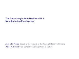
The Surprisingly Swift Decline of U.S. Manufacturing Employment. Justin R. Pierce, Board of Governors of the Federal Reserve System Peter K. Schott, Yale School of Management & NBER. Disclaimer

E N D
The Surprisingly Swift Decline of U.S. Manufacturing Employment Justin R. Pierce, Board of Governors of the Federal Reserve System Peter K. Schott, Yale School of Management & NBER
Disclaimer Any opinions and conclusions expressed herein are those of the authors and do not necessarily represent the views of the U.S. Census Bureau, the Board of Governors or its research staff. All results have been reviewed to ensure that no confidential information is disclosed.
Introduction • U.S. manufacturing employment declined sharply starting in 2001
Post-War U.S. Manufacturing Employment U.S. manufacturing employment reached a peak of 19.5 million in 1979 Source: Pierce and Schott (2012)
Post-War U.S. Manufacturing Employment In the following 22 years, it fell 2.6 million Source: Pierce and Schott (2012)
Post-War U.S. Manufacturing Employment In the next 30 months, it fell 2.7 million… Source: Pierce and Schott (2012)
Post-War U.S. Manufacturing Employment In the next 30 months, it fell 2.7 million… …faster than in the Great Recession Source: Pierce and Schott (2012)
Introduction • Trade liberalization is often blamed for the loss of manufacturing jobs • We investigate the link between the post-2001 decline and a specific change in policy • China’s receipt of permanent normal trade relations (PNTR) from the US and its subsequent entry into the WTO • PNTR-WTO did not change tariff rates but it did eliminate trade policy uncertainty by reducing the risk of tariff increases
Before Continuing… Our goal is to understand the post-2001 decline We do not attempt a welfare analysis of PNTR Source: Pierce and Schott (2012)
Outline • US-China Trade Policy • Data • Employment • NTR gaps • Results • Industries • Plants • Trade
Basic Tariff Nomenclature • NTR = Normal Trade Relations • New term for Most Favored Nation (MFN) • The US has two basic sets of tariffs • NTR tariffs: for WTO members • Non-NTR tariffs : for non-WTO members (historically applied to non-market economies) • Non-NTR rates originally set in Smoot-Hawley Tariff Act (1930) • Non-NTR tariffs are generally higher, sometimes substantially
U.S.-China Trade Policy, 1980-2001 2001 (December) China enters WTO Annual renewals were uncertain, especially after the Tiananmen Square incident in 1989 (e.g., the House passed resolutions of disapproval in 1990, 1991 and 1992, though the Senate failed to act on them) 1980 (February) China was granted temporary NTR status (TNTR) by the US Congress TNTR required annual re-approval by Congress 2000 (October) U.S. Congress grants China PNTR, eliminating uncertainty
Measuring Trade Policy Uncertainty • We measure uncertainty under TNTR as the amount by which tariffs would increase if re-approval were rejected by Congress • For product p, this increase is: NTR Gapp= Non-NTR Tariffp – NTR Tariffp • We use a difference-in-differences strategy to compare industry and plant outcomes after 2001 with outcomes after the prior 2 NBER peaks (1981 and 1990) • Raw, publicly available data provide a preview of our results • Split industries according to the median NTR Gapi • Examine employment trends before and after 2001
Preview of Findings - Employment Source: Pierce and Schott (2012)
Preview of Findings – Employment by Labor Intensity Capital-intensive industries Source: Pierce and Schott (2012)
Preview of Findings – Employment by Labor Intensity Labor-intensive industries Source: Pierce and Schott (2012)
Preview of Findings – Employment by Labor Intensity Trends are similar among both capital-intensive and labor- intensive industries Source: Pierce and Schott (2012)
Preview of Findings - Trade U.S. imports from China grow disproportionately in high-gap products Source: Pierce and Schott (2012)
Preview of Findings - Trade U.S. imports from China grow disproportionately in high-gap products No similar trend in ROW imports Source: Pierce and Schott (2012)
Related Research • Employment and trade liberalization • Lots of papers • Autor et al. (2012); Bloom et al. (2012); Groizard et al. (2012) • Investment under uncertainty • Lots of papers • Trade: Handley (2012); Handley and Limao (2012) • “Jobless” recoveries • Manufacturing: Faberman (2012) • Overall: Jaimovich and Siu (2012) • Supply-chain linkages • US manufacturing: Ellison, Glaeser and Kerr (2010) • Trade: Baldwin and Venables (2012)
Outline • US-China Trade Policy • Data • Employment • NTR Gaps • Results • Industries • Plants • Trade
Data 1: Establishment-Level Employment LBD • Longitudinal Business Database • Annual, 1977-09 • All private establishments • Observe • “Major industry” • Employment (as of March) CM • Census of Manufactures • Every 5 years, 1972-07 • Manufacturing plants • Observe • “Major industry” • Production and non-production workers • Shipments • Value added • Capital stock (book value)
We Construct a Constant ManufacturingSample • Issues with raw LBD/CM manufacturing data • SIC g NAICS in 1997 • Activities considered “manufacturing” change within and across SIC and NAICS over time • We use various concordances to create “families” of four-digit SIC and six-digit NAICS industries that collect similar activities over time • Yields 363 families in manufacturing • From here forward, “industry” generally refers to “family” • We make two drops for any time interval we examine • Drop families containing non-manufacturing activities • Drop plants that transition between manufacturing and non-manufacturing
Constant-Manufacturing LBD vs BLS LBD BLS We use the LBD to compare employment growth up to 6 years after the 1981, 1990 and 2001 NBER peaks Note: Data are annual as of March.
Data 2: NTR Gaps • For eight-digit HS product pand year tcompute NTR Gappt = Non-NTR Tariffpt – NTR Tariffpt using Feenstraet al. (2001) ad valorem equivalent tariff schedule for 1989-2001 • Higher gap g greater potential tariff hike under TNTR • For industry-level CM and LBD data, average product-level gaps to industries NTR Gapi = mean(NTR Gapp) p in i
Distribution of NTR Gaps Over IndustriesBy Year, 1989-2001 We use the gap for 1999 in the results to follow, but results are robust to using any year
Outline • PNTR and theoretical motivation • Data • Employment • NTR Gaps • Empirical Strategy and Results • Industries • Plants • Trade
Industry-Level OLS Diff-in-Diff(i=industry; t=NBER peak; d=years after peak) Peak-year and industry fixed effects Interaction of indicator variable for 2001 peak and time-invariant NTR Gap Industry attributes Cumulative percent change in industry i employment d years after NBER peak t={1981,1990,2001} • Features • Estimate this equation separately for d=1:6 • Compare outcomes within industries across business cycles • Remove average growth d years after peak to control for cyclicality
Industry-Level RegressionsBold=statistically significant at 10% level
Industry-Level RegressionsBold=statistically significant at 10% level Cumulative industry employment growth as percent of initial level for 1981-1987, 1990-1996 and 2001-2007
Industry-Level RegressionsBold=statistically significant at 10% level Cumulative industry employment growth as percent of initial level for 1981-1987, 1990-1996 and 2001-2007 There are 363 “families” per year NBER peak
Industry-Level RegressionsBold=statistically significant at 10% level • NTR gap is negative and statistically significant at 10 percent level for d=1:6 • Absolute magnitude of coefficient rises over time; losses are persistent
Industry-Level RegressionsBold=statistically significant at 10% level • NTR gap is negative and statistically significant at 10 percent level for d=1:6 • Absolute magnitude of coefficient rises over time; losses are persistent • Multiply coefficient above by average NTR gap to assess implied impact of PNTR • Post-2001 growth is -4.1 to -17.8 percentlower relative to prior recoveries
Industry-Level RegressionsBold=statistically significant at 10% level Final column uses CM rather than LBD CM regression compares 1997-07 to 1977-87 and 1987-97 With CM, we can control for industry capital (K) and skill (NP workers) intensity Effect for 1997-2007 similar to 2001-2007; decline concentrated after 2001
Industry-Level RegressionsBold=statistically significant at 10% level Final column uses CM rather than LBD CM regression compares 1997-07 to 1977-87 and 1987-97 With CM, we can control for industry capital and skill intensity Effect for 1997-2007 similar to 2001-2007; decline concentrated after 2001
Margins of Adjustment • Benefit of plant-level data is the ability to analyze gross intensive and extensive margins of adjustment • Here, one intensive and two extensive margins • PE,PC: expanding, contracting plants at continuing firms • PB,PD: plant birth, death in continuing firms • FB,FD: firm birth and death • Compute cumulative percent change in employment along each margin (m) as a share of initial industry level: Growth across the six gross margins sums to the overall growth of the industry
Margins of Adjustment • Benefit of plant-level data is the ability to analyze gross intensive and extensive margins of adjustment • Here, one intensive and two extensive margins • PE,PC: expanding, contracting plants at continuing firms • PB,PD: plant birth, death in continuing firms • FB,FD: firm birth and death • Compute cumulative percent change in employment along each margin (m) as a share of initial industry level: Job Creation Job Destruction
Implied Impact of PNTR(by Job Creation vs Job Destruction) • Faberman (2012): joblessness of 2001 recover due to shift down in job creation shift up in job destruction • Here, we find that both of these shifts are related to PNTR • Contribution of anemic job creation rises over time, as jobs that “normally” are created after 1981 and 1990 do not come back after 2001 Relative importance of low job creation rises over time
Coarse Counterfactual • We construct a coarse counterfactual of effect of PNTR on employment using the above industry-level estimates • Multiply coefficients for each margin by the corresponding gap for each industry • Compute estimated job loss from exaggerated job destruction (JD) and anemic job creation (JC) • Sum these estimates over industries and add back to actual employment loss
Coarse Counterfactual Add Back Estimated Job Creation and Destruction Add Back Estimated Job Destruction Actual Loss
Coarse Counterfactual Add Back Estimated Job Creation and Destruction Add Back Estimated Job Destruction Actual Loss
Upstream and Downstream NTR Gaps • PNTR may also have an effect through input-output linkages • Lower prices of Chinese imports used as inputs may lead an industry to enjoy increased output and employment • Displacement of downstream customers may lead an industry to suffer decreased output and employment • Supply chain research (e.g. Baldwin and Venables2012) • Relocation of customers or suppliers may lead to relocation of a discrete chunk of a supply chain • We construct upstream and downstream gaps using weights from BEA’s 1997 Benchmark Input-Output Tables • (See paper for details)
Industry-Level RegressionsBold=statistically significant at 10% level
Industry-Level RegressionsBold=statistically significant at 10% level
Industry-Level RegressionsBold=statistically significant at 10% level