Download
1 / 43
430 likes | 522 Vues
Explore condensation in horizontal microchannels for automotive AC & petrochemicals. Enhance heat transfer & decrease ozone-depleting fluid use. Learn prediction models like Friedel (1979; 1980) and Chen (2001) for pressure drop & optimization. Study related factors, Reynolds numbers, friction, and gradients for efficient heat and mass transfer applications. Benefit from research by experts in the field.

E N D
Condensation in mini- and microchannels Hussein Dhanani Sebastian Schmidt Christian Metzger Assistant: Marcel Christians-Lupi Teacher: Prof. J.R Thome 20 December 2007 Heat and Mass Transfer Laboratory
Structure • Introduction to condensation in microchannels • Pressure drop • Prediction models • Friedel (1979;1980) • Chen (2001) • Cavallini (2001;2002) • Wilson (2003) • Garimella (2005) • Graph analysis Heat and Mass Transfer Laboratory
Structure • Heat transfer • Prediction models • Shah (1979) • Dobson & Chato (1998) • Cavallini (2002) • Bandhauer (2005) • Graph analysis • Questions Heat and Mass Transfer Laboratory
Introduction • Condensation inside horizontal microchannels • Automotive air-conditioning, petrochemical industry • Reduce use of ozone-killing fluids • Increase heat transfer coefficient and pressure drop • Surface tension + Viscosity>>> gravitational forces Heat and Mass Transfer Laboratory 4
Pressure drop • Common parameters used by several correlations • Liquid Reynolds number • Vapor Reynolds number • Liquid-only Reynolds number • Vapor-only Reynolds number Heat and Mass Transfer Laboratory
Pressure drop • Common parameters used by several correlations • Single-phase friction factor (smooth tube) • Single-phase pressure gradients Heat and Mass Transfer Laboratory
Pressure drop prediction models • Friedel (1979;1980) • Considered Parameters • Liquid only single-phase pressure gradient • Liquid only and vapor only friction factor • Fluid and geometric properties • Range / applicability • D > 1 mm • Adiabatic • μl/μv < 1000 Heat and Mass Transfer Laboratory
Pressure drop prediction models • Friedel (1979;1980) Heat and Mass Transfer Laboratory
Pressure drop prediction models • Chen et al. (2001) • Modification of the Friedel correlation by adding two-phase multiplier • Considered Parameters • Two-phase pressure gradient by Friedel • We, Bo, Rev, Relo • Range / applicability • 3.17 < D < 9 mm for R-410A • 5°C < Tsat < 15°C • 50 < G < 600 kg/m2s Heat and Mass Transfer Laboratory
Pressure drop prediction models • Chen et al. (2001) Heat and Mass Transfer Laboratory
Pressure drop prediction models • Cavallini et al. (2002) • Modification of the Friedel correlaction for annular flow. • Considered Parameters • Liquid only single-phase pressure gradient • Liquid only and vapor only friction factor • Fluid and geometric properties • Range / applicability • D = 8 mm for R-134a , R-410a and others • 30°C < Tsat < 50°C • 100 < G < 750kg/m2s Heat and Mass Transfer Laboratory
Pressure drop prediction models • Cavallini et al. (2002) Friedel Heat and Mass Transfer Laboratory
Pressure drop prediction models • Cavallini et al. (2002) Heat and Mass Transfer Laboratory
Pressure drop prediction models • Wilson et al. (2003) • Considered parameters • Single-phase pressure gradients (liquid-only) • Martinelli parameter • Range / applicabilty • Flattened round smooth, axial, and helical microfin tubes. • 1.84 < D < 7.79 mm for R-134a, R-410A • Tsat = 35°C • 75 < G < 400 kg/m2s Heat and Mass Transfer Laboratory 14
Pressure drop prediction models Model uses liquid-only two-phase multiplier of Jung and Radermacher (1989): Xtt is the Martinelli dimensionless parameter for turbulent flow in the gas and liquid phases. Insert formulation • Wilson et al. (2003) Heat and Mass Transfer Laboratory 15
Pressure drop prediction models Knowing the single-phase pressure gradient, the two-phase pressure grandient is: with Single-phase friction factors are calculated using the Churchill correlation (1977): • Wilson et al. (2003) Heat and Mass Transfer Laboratory 16
Pressure drop prediction models • Garimella et al. (2005) • Considered parameters • Single-phase pressure gradients • Martinelli parameter • Surface tension parameter • Fluid and geometric properties • Range / applicabilty • 0.5 < D < 4.91 mm for R-134a • Tsat ~ 52°C • 150 < G < 750 kg/m2s Heat and Mass Transfer Laboratory 17
Pressure drop prediction models Void fraction is calculated using the Baroczy (1965) correlation: Liquid and vapor Re values are given by: • Garimella et al. (2005) Heat and Mass Transfer Laboratory 18
Pressure drop prediction models Liquid and vapor friction factors: Therefore, the single-phase pressure gradients are given and the Martinelli parameter is calculated: • Garimella et al. (2005) Heat and Mass Transfer Laboratory 19
Pressure drop prediction models Liquid superficial velocity is given by: This velocity is used to evaluate the surface tension parameter: • Garimella et al. (2005) Heat and Mass Transfer Laboratory 20
Pressure drop prediction models Interfacial friction factor: Laminar region: Turbulent region (Blasius): • Garimella et al. (2005) Heat and Mass Transfer Laboratory 21
Pressure drop prediction models The pressure gradient is determined as follows: • Garimella et al. (2005) Heat and Mass Transfer Laboratory 22
Pressure drop prediction models G = 400 kg/m2s G = 800 kg/m2s Tsat = 40°C , D = 1.4 mm • Graph analysis for R-134a Heat and Mass Transfer Laboratory 23
Pressure drop prediction models G = 600 kg/m2s G = 1000 kg/m2s Tsat = 40°C , D = 1.4 mm • Graph analysis for R-410A Heat and Mass Transfer Laboratory 24
Heat transfer • Common parameters used by several correlations • Prandtl number • Reduced pressure • Martinelli parameter Heat and Mass Transfer Laboratory 25
Heat transfer prediction models • Shah (1979) • Considered parameters • Vapor Velocity • Liquid-only Reynolds number • Liquid Prandtl number • Reduced pressure • Fluid and geometric properties • Range / applicability • 7 < D < 40 mm • Various refrigerants • 11 < G < 211 kg/m2s • 21 < Tsat < 310°C Heat and Mass Transfer Laboratory 26
Heat transfer prediction models Applicability range: If range is respected, compute liquid-only transfer coefficient: • Shah (1979) Heat and Mass Transfer Laboratory 27
Heat transfer prediction models For heat transfer coefficient, apply multiplier: Widely used for design. Improvement needed for results near critical pressure and vapor quality from 0.85 to 1. • Shah (1979) Heat and Mass Transfer Laboratory 28
Heat transfer prediction models • Dobson and Chato (1998) • Considered parameters • Liquid, vapor-only Reynolds number • Martinelli parameter • Zivi’s (1964) void fraction • Galileo number • Modified Soliman Froude number • Liquid Prandtl number • Range / applicability • D = 7.04 mm • 25 < G < 800 kg /m2s • 35 < Tsat < 60°C Heat and Mass Transfer Laboratory 29
Heat transfer prediction models Calculate the modified Soliman Froude number: • Dobson and Chato (1998) Heat and Mass Transfer Laboratory 30
Heat transfer prediction models With: • Dobson and Chato (1998) Heat and Mass Transfer Laboratory 31
Heat transfer prediction models For Frso > 20, the annular flow correlation proposed is And the resulting heat transfer coefficient is: • Dobson and Chato (1998) Heat and Mass Transfer Laboratory 32
Heat transfer prediction models • Cavallini et al. (2002) Applicable for annular regime only • Considered Parameters • Pressure drop • Dimensionless film thickness • Dimensionless temperature • Re, Pr • Fluid and geometric properties • Range / applicability • D = 8 mm • R134a and R410a • 100 < G < 750 kg/m2s • 30 < Tsat < 50°C Heat and Mass Transfer Laboratory 33
Heat transfer prediction models • Calculation of the shear stress • Dimensionless film thickness Heat and Mass Transfer Laboratory 34
Heat transfer prediction models • Heat transfer coefficient Heat and Mass Transfer Laboratory • Dimensionless temperature 35
Heat transfer prediction models • Bandhauer et al. (2005) • Considered parameters • Pressure drop • Dimensionless film thickness • Turbulent dimensionless temperature • Pr • Fluid and geometric properties • Range / applicability • 0.4 < D < 4.9 mm • R134a • 150 < G < 750 kg/m2s Heat and Mass Transfer Laboratory 36
Heat transfer prediction models Interfacial shear stress: Friction velocity is now calculated: • Bandhauer et al. (2005) Heat and Mass Transfer Laboratory 37
Heat transfer prediction models Film thickness is directly calculated from void fraction: This thickness is used to obtain the dimensionless film thickness: • Bandhauer et al. (2005) Heat and Mass Transfer Laboratory 38
Heat transfer prediction models Turbulent dimensionless temperature is given by: Therefore, the heat transfer coefficient is: • Bandhauer et al. (2005) Heat and Mass Transfer Laboratory 39
Heat transfer G=175 kg/m2s G=400 kg/m2s D=2.75mm, Tsat=35°C Heat and Mass Transfer Laboratory • Graph analysis for R134a 40
Heat transfer G=175 kg/m2s G=400 kg/m2s D=2.75mm, Tsat=35°C Heat and Mass Transfer Laboratory • Graph analysis for R410a 41