Lecture 23. State Space I

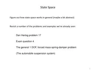
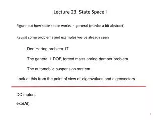
1. Lecture 23. State Space I Figure out how state space works in general (maybe a bit abstract) Revisit some problems and examples we’ve already seen Den Hartog problem 17 The general 1 DOF, forced mass-spring-damper problem The automobile suspension system Look at this from the point of view of eigenvalues and eigenvectors DC motors exp(At)

2. We care about this because it is a major tool for our design of controls

3. QUICK EXAM COMMENTS I graded on a four point scale and the mean was 9.8/16 The top score was 15/16 and the bottom score 0/16 I put them in your file folders before break If you got fewer than 8 points, you should probably be somewhat concerned The solution to the last problem given in the solution set is wrong Let me take two slides to give the right answer

4. m q l M y

5. Energies Constraints The Lagrangian Euler-Lagrange equations

6. The idea of state space is to go from one or more second order ODEs to twice as many first order ODEs We do this by doubling the number of variables by treating the first derivatives of the generalized coordinates as variables In equation form this is essentially a definition of p This makes We know what equals; we found it when we found the equations of motion Let’s call it

7. Suppose we start with the Euler-Lagrange equations In most cases it is relatively easy to convert them to the form where the Ps are linear combinations of the Qs, that may depend on the qs Then we can write

8. I have twice as many equations in twice as many unknowns, but the equations are all first order equations, and we’ll see how good that is I can define a state vector and a vector for its rate of change (the right hand side of the equations at the bottom of the previous slide) The differential equations in vector form become these are functions of p and q

9. Note that this equation is not necessarily linear because the gs may be nonlinear

10. Let me introduce a matrix B to allow me to split P from the right hand side and rewrite the differential equation as

11. Under circumstances for which the system is linear or for which it makes sense to linearize the system we get the following very nice-looking matrix equation for a single input system we’ll have where u denotes the input This is not the same A that we had before. We get it by inspection, and we’ll learn how

12. How do we solve this? We can look at this as a matrix analog of scalar solutions you already know It will get a little intricate, please bear with me as we go I will look at this a few times today

13. The scalar analog We can write rearrange integrate multiply rearrange

14. So that we see that the scalar analog has the solution which we can verify by direct substitution Add them up and cancel equal and opposite terms NOTE THAT THIS IS NOT A STABLE SOLUTION UNLESS A < 0

15. The vector problem Has an analogous solution We will see later what the exponent of a matrix is; we don’t need it for now, because we can solve simple problems without it

16. Once we have the system we can proceed as before Find a homogeneous solution that satisfies we can reduce that problem to the matrix eigenvalue problem Find a particular solution that satisfies The nature of this depends on the nature of f Combine the two through the initial condition

17. We can embed this process in what we know so far Find the energies, the Lagrangian and the Euler-Lagrange equations including the dissipation and any generalized forces Linearize if necessary Convert to state space Find a homogeneous solution that satisfies which we can reduce to the matrix eigenvalue problem Find a particular solution that satisfies Combine the two through the initial condition Finally we need to interpret x back in the physical world from which the problem came

18. QUESTIONS?

19. You’ve put up with several abstract slides Let’s take a look at how one actually addresses this in specific cases We’ll look at things we’ve already seen, at least at first The one degree of freedom problem Den Hartog problem 17 The general 1 DOF, forced mass-spring-damper problem A two degree of freedom auto suspension model

20. The simplest case Look at the 1 DOF equation of motion Let Then Or

21. For this example: QUESTIONS?

22. Den Hartog problem 17 2klsinq fR klsinq q mg mg A mg

23. combine terms linearize the equation of motion

24. Get rid of the constant term, which represents the sag of the system under gravity Write the operative part of the equation does NOT involve gravity We’ll tackle this in state space

25. What do we do in state space? We can drop the primes as no longer necessary and write define then

26. This is a homogeneous problem, so we only have a wee bit of work to do to solve it Seek exponential solutions so This is the matrix eigenvalue problem

27. the determinant that must vanish is The two roots are the eigenvalues of A

28. Our rule for eigenvectors gives us and we can assemble the general homogeneous solution

29. Suppose we start from rest with an angle offset of π/20 small enough that the linear approximations will be OK The initial condition for x will be initial angle initial speed

30. We can decompose this to identify the angle and its rate of change which is, of course, exactly what we expect to find: the state space result makes sense!

31. QUESTIONS?

32. mass-spring-damper system m c f k This one follows the same pattern

34. damping ratio (which I will suppose < 1 in later work) natural frequency General one degree of freedom equation

37. We get the eigenvectors for each eigenvalue by substituting the eigenvalues The homogeneous solution

38. Let’s take our old friend harmonic forcing and look at the particular solution choosing A to be real fixes the phase of the forcing (cosine)

40. Plug all this in I’m going to grind through taking the real part of this this one time Multiply top and bottom by the complex conjugate and we have

41. Factor out stuff that is real to make it easier to see what is going on Expand the product

43. Now we can look at the initial condition and let’s start from rest Add these and evaluate at t = 0

44. We can solve these for a and b, but the algebra is a bit daunting to put up on screen (and to type out), so here is the Mathematica result

46. The homogeneous solution is then made up of the appropriate amounts of each eigenvector and eigenfunction eigenfunctions eigenvectors You can expand this by hand, but it’s quite messy because a and b are complex

48. QUESTIONS?

49. From Gillispie, TD Fundamentals of Vehicle Dynamics (1992) We can fit this to our vertical model

50. Rotate our picture to the vertical c2 k2 z2 f2 m2 c3 k3 f1 z1 m1 c1 k1