Observation Operators in Variational Data Assimilation

Observation Operators inVariational Data Assimilation David Tan, Room 1001 (David.Tan@ecmwf.int) Angela Benedetti (Angela.Benedetti@ecmwf.int) Thanks to Erik Andersson, Philippe Lopez and Tony McNally

Plan of Lecture • Why do we need observation operators? • The link to enable comparison of model with observations • Different components of observation operators • From “well-established” to “exotic” • Jacobians (linearized operators) • Starting point for understanding information content • Why variational schemes are very flexible with respect to data usage • They overcome several “retrieval problems” • Summary • Recap typical issues arising with observation usage

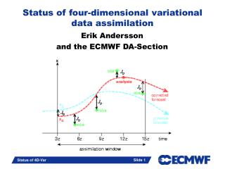
Reminder of 4D-Var Characteristics • ECMWF’s 4D-Var uses a wide variety of observations: both conventional (ground-based or aircraft) and satellite data • All data within a 12-hour period are used simultaneously, in one global (iterative) estimation problem • 4D-Var finds the 12-hour forecast evolution that is a best fit (or at least a compromise) between the previous “background” forecast and the newly available observations • It does so by adjusting 1) surface pressure, and the upper-air fields of 2) temperature, 3) winds, 4) humidity and 5) ozone (and, in research mode, other tracers) Observation operators provide the linkto enable comparison of model with observations

The observation operator “H” • How to compare model with observations? Satellites measure radiances/brightness temperatures/reflectivities, etc., NOT directly temperature, humidity and ozone. • A model equivalent of the observation needs to be calculated to enable comparison in observation space (or related model-equivalent space). • This is done with the ‘observation operator’, H. • H may be a simple interpolation from model grid to observation location for direct observations, for example, of winds or temperature from radiosondes • H may possibly perform additional complex transformations of model variables to, for example, satellite radiances: Model T,u,v,q,o3 Compare Observed satellite radiance Model radiance H O-B Obs-Background (also O-A)

Model T and q Observed satellite radiance Model radiance H compare Forecast versus observed fields Meteosat imagery – water vapour channel

Observation operator versus retrievals • What about transforming observations closer to model space? Is possible to use “satellite retrievals” BUT often involves many modelling assumptions. Presents different set of difficulties for assimilation. • H becomes simpler for a satellite retrieval product • Related tangent linear & adjoint operators also simpler • Retrieval assumptions made by data providers not always explicit/valid • Use of NWP data in retrieval algorithms can introduce correlated errors Satellite retrieval e.g. o3, aod, AMV, hlos Retrieval algorithm Model T,u,v,q,o3 Model equivalent Observed satellite quantity H O-B Units of mixing ratio, m/s etc Model equivalent Model T,u,v,q,o3 Observed satellite quantity H O-B Units of radiance

Observational data There is a wide variety of observations, with different characteristics, irregularly distributed in space and time. So there is also a wide variety of observation operators Quick quiz: what range of operations do we need to compare with the shown observations?

Comparing model and observations • The forecast model provides the background (or prior) information to the analysis • Observation operators allow observations and model background to be compared (“O-B”) • The differences are called departures or innovations • They are central in determining the most likely correction to the model fields • These corrections, or increments, are added to the background to give the analysis (or posterior estimate) • Observation operators also allow comparison of observations and the analysis (analysis departures “O-A”)

Statistics of departures = observations Background departures: Analysis departures: (O-B) (O-A) = analysis state = background state Aircraft temperature Radiosonde temperature • The standard deviation of background departures for both radiosondes and aircraft is around 1-1.5 K in the mid-troposphere. • The standard deviation of the analysis departures is approximately 30% smaller – the analysis has “drawn” to the observations.

Statistics of departures = observations First guess departures: Analysis departures: (O-B) (O-A) = analysis state = background state Aircraft temperature Radiosonde temperature • Such statistics provide feedback on the assimilation system, but also on the forecast model and on observation quality • Bias(departures) = bias(obs) – bias(model) • Variance(departures) = variance(obs) + variance(model) • When model and observation quality can be separated, data assimilation can give useful feedback to model developers and data providers

Formalism of variational estimation The variational cost function J(x) consists of a background term and an observation term involving the observation operator H The relative magnitude of the two terms determines the size of the analysis increments. The solution in the linear case (H=H) is: increment Departures (in general 4d-Var uses nonlinear H here!) y:array of observations x:represents the model/analysis variables H:linearized observation operators B:background error covariance matrix R:observation error covariance matrix Background error covariance in terms of the observed quantities

Definition of ‘observation operator’ The observation operator provides the link between the model variables and the observations (Lorenc 1986; Pailleux 1990). The symbol H in the variational cost-function signifies the sequence of operators transforming the analysis control variable x into the equivalents of each observed quantity y, at observation locations. This sequence of operators can be multi-variate and may include: • “Interpolation” from forecast time to observation time (in 4D-Var this is actually running the forecast model over the assimilation window) • Horizontal and vertical interpolations • Vertical integration • If limb-geometry, also horizontal integration • If radiances, radiative transfer computation • Any other transformation to go from model space to observation space.

Actual specification of observation operators used in the ECMWF 4D-Var The operator H in the variational cost-function signifies a sequence of operators. Each one performs part of the transformation from control variable to observed quantity: • These first three steps are common for all data • types: • The inverse change of variable converts from control variables to model variables • The inverse spectral transforms put the model variables on the model’s reduced Gaussian grid • A 12-point bi-cubic horizontal interpolation gives vertical profiles of model variables at observation points • Further steps: • Vertical interpolation to the level of the observations. The vertical operations depend on the observed variable • Verticalintegration of, for example, the hydrostatic equation to obtain geopotential, and of the radiative transfer equation to obtain top of the atmosphere radiances. Change of variable Forecast Inverse transforms Forward Horizontal interpolation Adjoint Vertical interpolation Radiative transfer Jo-calculation

Upper-air observation operators The following vertical interpolation techniques are employed: Wind: linear in ln(p) on full model levels Geopotential: as for wind, but the interpolated quantity is the deviation from the ICAO standard atmosphere Humidity: linear in p on full model levels Temperature: linear in p on full model levels Ozone: linear in p on full model levels

Interpolation of highly nonlinear fields • The problem of a “correct” horizontal interpolation is especially felt when dealing with heterogeneous model fields such as precipitation and clouds. • In the special case of current rain assimilation, model fields are not interpolated to the observation location. Instead, an average of observation values is compared with the model-equivalent at a model grid-point – observations are interpolated to model locations. • Statistics on next slide all use the same model & the same observations, the only change is the horizontal interpolation in the observation operator. • Different choices can affect the departure statistics which in turn affect the observation error assigned to an observation, and hence the weight given to observations.

4D-Var rain/cloud treatment of grid-point – observation problem SSM/I T511 Slide courtesy of P.Lopez

4D-Var rain/cloud treatment of grid-point – observation problem SSM/I T159 Slide courtesy of P.Lopez

Representativeness Errors • Errors introduced by the interpolation operator, and also by the finite resolution of the model fields, are often accounted for by adding “representativeness” errors to the “instrument” error of the observations. • For some data, e.g. radiosonde winds, the representativeness errors are the dominant contribution to the observation errors in the matrix R. Equivalently, normally accounted for in estimates of observation error variance in departure statistics – recall Variance(departures) = variance(obs) + variance(model) • In effect, we compare model and observations not in observation space, but in model-equivalent space. We ask what would the observed quantity be if we degraded the atmosphere down to model resolution?

Radiative transfer operator* Satellite instruments (active and passive) simply measure the RADIANCEL that reaches the top of the atmosphere at given frequency v . The measured radiance is related to geophysical atmospheric variables (T,Q,O3) by the radiative transfer equation (covered in detail in other lectures). Surface emission Surface reflection/ scattering Cloud/rain contribution + + + +... The observation operator for satellite measurements is in this case a convolution of the horizontal and vertical interpolation operators and the radiative transfer equation applied to the interpolated model state variables (for example, temperature, humidity) and solved via approximations which depend on the specific channel/frequency. * Details in presentations by T. McNally and M. Matricardi

Example of a radiative transfer operator* RT for atmospheric sounding channels • These channels are located in parts of the infra-red and microwave spectrum for which the main contribution to the measured radiance is from the atmosphere and can be written: Where B=Planck function = transmittance T(z) is the temperature z is a height coordinate • They are chosen to avoid frequencies for which surface radiation and cloud • contributions are important, and are primarily used to obtain information • about atmospheric temperature and humidity (or other constituents that • influence the transmittance e.g. CO2). * Details in presentations by T. McNally and M. Matricardi

Surface observation operators The operators for 10m wind and 2m temperature are based on Monin-Obukhov similarity theory to match an earlier version of the physical parametrisation of the forecast model Auxiliary parameters These are inputs which are not updated i.e. assumed fixed Updated by the analysis, i.e. part of the control variable

“Unusual” observation operators (I) (research-only, not operational) Aerosol optical depth (AOD): • The operator is based on tabulated or parameterized optical properties of the N aerosol species that are modeled. These optical properties are then weighted by the mass of the particulate to provide the extinction coefficient and integrated vertically to give the total optical depth at a given wavelength: where is the extinction coefficient which is a function of particle size and height (and relative humidity for some aerosol types). • An aerosol optical depth operator is currently used in the project “Monitoring of the Atmospheric Composition and Climate” (MACC) for the assimilation of the Moderate Resolution Imaging Spectroradiometer (MODIS) aerosol optical depths at 550 nm.

“Unusual” observation operators (II)(research-only, not operational) Radar reflectivity: • Radar reflectivity, Z, is related to radar backscattered power. The standard definition is as follows where N is the number density of the cloud/rain droplets and D is their diameter. • For practical applications, tabulated values of radar reflectivity are computed and stored as functions of liquid/ice water content or precipitation (snow/rain) and temperature • Used in retrievals/assimilation of cloud properties, or surface precipitation (depends on the frequency of the radar, 94/35 GHz for clouds and light precipitation, 14/10 GHz for precipitation). • Experimentally, the radar data from the US network (NEXRAD) have been tested for assimilation of surface precipitation in the ECMWF system (P. Lopez). A version of this operator is currently being adapted to use CloudSAT data (and potentially EarthCARE in future).

Backscatter signal • Aeolus winds are derived from Doppler shift of aerosols and molecules along lidar line-of-sight • Error estimates, cloud & aerosol properties derived from signal strength Background for ADM-AeolusDopplier Wind Lidar - Measurement Concept CALIPSO lidar – vertical cross sections of backscatter

Background for ADM-AeolusGeometry for measuring horizontal wind UV lidar (355 nm) with two receivers - Mie (aerosol), Rayleigh (molecules) - both use direct detection Wind profiles from surface to 30 km with resolution varying from 0.5 to 2 km - vertical bins configurable in flight - HLOS component only - direction 7º from zonal at equator - 6 hour coverage shown Burst mode 1 obs ~ 50 meas Scalable system

Key assimilation operators for DWL hlos • HLOS, TL and AD • H = - u sin φ - v cos φ • dH = - du sin φ - dv cos φ • dH* = ( - dy sin φ, - dy cos φ )T • φ is azimuth angle measured from North • Generalize to layer averages later • Background error • Same as for u and v (assuming isotropy) • Assumes good quality retrieval algorithms to obtain hlos from Level-1B backscatter measurements (the lidar spectrometers measure interference fringes from transmitted and received signal) – ECMWF project 2005 to present

Background for ADM-AeolusOptical Receiver • Mie light reflected into Rayleigh channel • Rayleigh wind algorithm includes correction term involving scattering ratio (s) • To develop observation operators, retrieval algorithms and/or just to understand data (especially their limitations) it’s important to have some understanding of the instrument – in the case of Doppler Wind Lidar, the Optical Receiver that measures the interference fringes • Mie channel detects scattering from particles (aerosol, cloud) • Rayleigh (two sub-channels) detects scattering from air molecules Astrium Satellites

Windgeschwindigkeit = 100 m/s l = 355 nm l = 355 nm l = 355 nm + 0,2 pm For scattering by particles, wind proportional to horizontal shift of interferencce fringe 16 Pixel 16 Pixel ADM-Aeolus Doppler Wind Lidar - Mie Spectrometer Windgeschwindigkeit = 0 m/s

FP-A FP-B CCD: For scattering by molecules, wind proportional to intensity difference I(A) I(B) ADM-Aeolus Doppler Wind Lidar - Rayleigh Spectrometer Windgeschwindigkeit = 0 m/s Windgeschwindigkeit = 250 m/s I(A) I(B)

Lidars are active instruments • Lidar has enormous potential for many types of observations • Self-calibrating, low-bias, good vertical resolution • Clouds – CALIPSO, EarthCARE (regular backscatter lidar) • Wind – ADM-Aeolus (Doppler Wind Lidar, DWL) • Water vapour – via DIfferential Absorption Lidar (DIAL) • Chemical constituents – CO2 etc, also via DIAL • Refs for Spaceborne Doppler Wind Lidar + Assimilation • Baker et al 1995, BAMS • ESA 1999 Report for Assessment (Stoffelen et al 2005, BAMS) and 2007/8 Science Report • Weissman and Cardinali 2006, QJRMS • N. Zagar & co-authors, QJRMS & Tellus A • Tan & Andersson 2005, QJRMS • Tan et al 2007, QJRMS • Tan et al 2008, Tellus A (Special Issue on ADM-Aeolus)

The Jacobian matrix • The tangent linear of the observation operator H consists of the partial derivatives of H with respect to all of its inputs, expressing the variations of H in the vicinity of the background xb. • His sometimes referred to asthe Jacobianof H. If H varies significantly with xb then H isnon-linear. • Needed for the incremental formulation of 4d-Var (adjoint too). • But also, for complex observation operators, study of the Jacobian highlights observation sensitivities to input model variables at specific points (quantified as information content, effectively which model components have been “observed”). • In the case of radiances, for example, columns of H will express each channel’s ‘weighting function’ on the model geometry.

A Jacobian example: MSU-2 • The Jacobian for TOVS channel MSU-2 is shown in the leftmost diagram. It can be interpreted as a profile of weights for a vertically averaged temperature. • The second diagram on the left shows the analysis increment in the special case of a diagonal B-matrix. • The two panels to the right show theoretical and actual analysis increments, with a realistic B-matrix. • Weighting functions and analysis increments are similar but not identical

Ambiguity The fact that some observations operators may be multivariate leads to ambiguity. In that case there is one observation - but many analysis components to correct. This is the classical retrieval problem, in its general form. Variational schemes resolve such ambiguities statistically, with the background (and its error characteristics in B) and the information from neighbouring observations as constraints. By contrast, retrieval products make additional assumptions so that only one “unknown” is solved for.

4D-Var as a retrieval scheme • One of the advantages of 3D/4D-Var is that it allows the direct assimilation of radiances and other “indirect” observations (e.g. optical depth, reflectivities, lidar backscatter): • Physical (based on radiative transfer calculations) • Simultaneous (in T, q, o3 and ps …) • Uses an accurate short-range forecast as background information, and its error covariance as a constraint • In 3D-Var: • Horizontal consistency is ensured • Other data types are used simultaneously • Mass-wind balance constraints are imposed • In 4D-Var: • Consistency in time. Frequent data can be used. • The dynamics of the model acts as additional constraint

Plan of Lecture • Why do we need observation operators? • The link to enable comparison of model with observations • Different components of observation operators • From “well-established” to “exotic” • Jacobians (linearized operators) • Starting point for understanding of information content • Why variational schemes are very flexible with respect to data usage • They overcome several “retrieval problems” • Summary • Recap typical issues arising with observation usage

Role of the observation operator H Every observed quantity that can be related to the model variables in a meaningful way, can be used in 3D/4D-Var. The link to enable the comparison of model and observations is the observation operator H • Accurately computing H(x) is important for deriving background departures and the assimilation’s analysis increments. Assumptions/approximations within the observational operator need to be taken into account, including the interpolation error and finite model resolution (they contribute representativeness error). • One observation can depend on several model quantities: Geop=H(T,Ps,q), Rad=H(T,q,o3,…). That is multi-variate. • H may be non-linear. Some TOVS channels vary strongly non-linearly with q (humidity), for example. Its first derivative H (the Jacobian) then depends on the atmospheric state. Moreover, when the observations are significantly influenced by geophysical quantities that are not currently analysed (e.g. surface emissivity, skin temperature, clouds or precipitation) then difficulties may arise.

Alternative approach to retrieval products The notion of ‘observation operators’ makes variational assimilation systems particularly flexible with respect to their use of observations. This has been shown to be of real importance for the assimilation of TOVS radiance data, for example. And it will be even more important in the coming years as a large variety of data from additional space-based observing systems become available - each with different characteristics. There is no need to convert the observed data to correspond to the model quantities. The retrieval is, instead, seen and integral part of the variational estimation problem.

Typical issues associated with observation usage • How can we compare the model to the observations? • Can we implement a forward operator H ? • Do we have all the information needed by the forward model? • How about the tangent linear and adjoint operators? • Are the operators computationally affordable? • Would it be better to use a retrieval product made elsewhere? • What additional assumptions are being made? Are they valid? • Can the processing assumptions/parameters be controlled? • There is often a transition from retrievals to lower-level products like radiances • Can take several years • How much weight should we give to the observations and background? • What are the sources of error? • Are the errors random or systematic? • Are bottom-up error budgets consistent with top-down? • Bottom up: instrument error, representativeness error, background error, model error • Top down: departure statistics, O-B and O-A • Answers from previous experience and further research • Even “old” observations need to be re-assessed

Supplementary slides

Options for grid-point – observation treatment Option 1: apply operator and interpolate output = IO Option 3: apply operator and take nearest output = NO Option 2: interpolate input and apply operator = II Option 4: take nearest input and apply operator = NI xi+1,j: +: TBi+1,j xi+1,j+1: +: TBi+1,j+1 xi+1,j+1: +: TBi+1,j+1 TBi,j=I(TBn) TBi,j=TBi+1,j+1 xi-1,j: +: TBi-1,j xi-1,j+1: +: TBi-1,j+1 xi+1,j+1 xi+1,j This is the option usually adopted in 4D-Var xi+1,j+1 xi,j=I(xn): +: TBi,j xi,j=xi+1,j+1: +: TBi,j xi-1,j xi-1,j+1 Operator: + = moist physics + microwave RT Slide courtesy of P.Lopez

More on representativeness errors • These may account for: • Errors in parameters defining the observation operator (e.g. prescribed • surface emissivity in radiative transfer) • Errors in the assumptions/simplifications used, and finite model resolution • Example: errors on optical depth due to the assumptions on type of mixing, • aerosol size and aerosol associated water can give an additional uncertainty of up to 32% in aerosol optical depth (Tsigaridis et al, 2008, ACPD)

More detail on aerosol model error computation (1) The 3 different aerosol mixtures Courtesy of Kostas Tsigaridis and Yves Balkanski

More detail on aerosol model error computation (2) Method to compute uncertatinties in optical parameters: • All particles are supposed spherical • Uncertainty on : optical depth, asymmetry parameter (g) and single scattering albedo (SSA) • 3 equally probable mixing states • Aerosol radius varies by ±20% by steps of 2% • Aerosol water varies by ±50% by steps of 5% • # cases = 3x21x21 = 1323 for each model box • These cases are used to determine a pdf (probability density function) • →From the pdf the uncertainty is determined as the range within which 68.2% (1s) and 95.4% (2s) of the cases considered fall respectively. Courtesy of Kostas Tsigaridis and Yves Balkanski

Observation Operators in Variational Data Assimilation