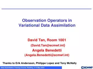
Observation Operators in Variational Data Assimilation
Observation Operators in Variational Data Assimilation. Erik Andersson Room: 302 Extension: 2627 erik.andersson@ecmwf.int. Plan of Lecture. Introduction The model and the observations Definition of “observation operator”, Multi-variate and non-linear

Observation Operators in Variational Data Assimilation
E N D
Presentation Transcript
Observation Operators inVariational Data Assimilation Erik Andersson Room: 302 Extension: 2627 erik.andersson@ecmwf.int DA/SAT Training Course, March 2006
Plan of Lecture • Introduction • The model and the observations • Definition of “observation operator”, • Multi-variate and non-linear • Why variational schemes are very flexible with respect to data usage • The principles of radiance assimilation DA/SAT Training Course, March 2006
A few 4D-Var Characteristics • ECMWF’s 4D-Var uses a wide variety of observations: both conventional and satellite data • All data within a 12-hour period are used simultaneously, in one global (iterative) estimation problem • 4D-Var finds the 12-hour forecast evolution that best fits the available observations • It does so by adjusting 1) surface pressure, and the upper-air fields of 2) temperature, 3) wind, 4) specifichumidity and 5) ozone Observation operators provide the linkbetween model and observations DA/SAT Training Course, March 2006
The observation operator • Observations are not made at model grid points • Satellites often measure radiances, NOT temperature, humidity and ozone • We calculate a model radiance equivalent of the observation to enable comparison. • This is done with the ‘observation operator’ H. • H may be a simple interpolation from model grid to observation location • H may possibly perform additional complex transformations of model variables to radiances for satellite data Model T,u,v,q,o3 Observed satellite radiance Model radiance H compare DA/SAT Training Course, March 2006
Model T and q Observed satellite radiance Model radiance H compare Forecast imagery versus observed DA/SAT Training Course, March 2006
ECMWF forecast model Vertical resolution 91 levels Observations are compared against a short-range 3-15 hour forecast Horizontal resolution TL799 ~ 25 km DA/SAT Training Course, March 2006
Observational data There is a wide variety of observations, with different characteristics, irregularly distributed in space and time. DA/SAT Training Course, March 2006
SYNOP/SHIP/METAR Ps, Wind-10m, RH-2m AIREP Wind, Temp SATOB Cloud Motion Winds DRIBU Ps, Wind-10m TEMP/DropSONDE Wind, Temp, Spec Humidity PILOT Wind profiles Profilers: Amer./Eu./Japan Wind profiles ATOVS and AIRS HIRS, AIRS and AMSU radiances SSM/I Microwave radiances (clear air) TCWV in rain and clouds Meteosat/MSG/GOES Water Vapour IR-channel QuikSCAT and ERS-2 Ambiguous winds-10m GOME/SBUV Ozone retrievals In preparation SSMIS, GPS-RO, GPS-ground based, Limb-sounding, ADM-Aeolus Data Used Conventional Satellite DA/SAT Training Course, March 2006
Comparing model and observations • The forecast model provides the background (or prior) information to the analysis • Observation operators allow observations and background to be compared • The differences are called departures or innovations • They are statistically combined to produce the most likely correction to the model fields • These corrections, or increments, are added to the background to form the analysis DA/SAT Training Course, March 2006
Example: temperature at 500 hPa 12-hour fc tendency 4D-Var analysis increment The corrections (or increments) are one order of magnitude smaller than the forecast 12-hour tendencies DA/SAT Training Course, March 2006
Statistics of departures (y-Hxb) Radiosonde temperature Aircraft temperature y-Hxb y-Hxa The standard deviation of background departures (y-Hxb) for both radiosondes and aircraft is around 1K in the mid-troposphere. Analysis departures (x-Hxa) are approximately 30% smaller. DA/SAT Training Course, March 2006
Definition of ‘observation operator’ The observation operators provide the link between the model variables and the observations (Lorenc 1986; Pailleux 1990). The symbol H in the variational cost-function signifies the ensemble of operators transforming the analysis control variable x into the equivalents of each observed quantity y, at observation locations. • Forecast to time of observation (in 4D-Var – not in 3D-Var) • Interpolations in horizontal and vertical • Vertical integration • If limb-geometry, also horizontal integration DA/SAT Training Course, March 2006
Formalism of variational estimation The variational cost function J(x) consists of a background term and an observation term The relative magnitude of the two terms determine the size of the analysis increments. The solution in the linear case is: increment y:array of observations x:represents the model/analysis variables H:linearized observation operators B:background error covariance matrix R:observation error covariance matrix departures Background error covariance in terms of the observed quantities DA/SAT Training Course, March 2006
Actual specification of 3D/4D-Varobservation operators The operator H in the variational cost-function signifies a sequence of operators. Each one performs part of the trans-formation from control variable to observed quantity: Change of variable The inverse change of variable converts from control variables to model variables The inverse spectral transforms put the model variables on the model’s reduced Gaussian grid A 12-point bi-cubic horizontal interpolation gives vertical profiles of model variables at observation points These first three steps are common for all data types Verticalintegration of for example the hydrostatic equation to form geopotential, and of the radiative transfer equation to form radiances Vertical interpolation to the level of the observations. The vertical operations depend on the observed variable Forecast Inverse transforms Forward Horizontal interpolation Adjoint Vertical interpolation Radiative transfer Jo-calculation DA/SAT Training Course, March 2006
Upper-air observation operators The following vertical interpolation techniques are employed Wind: linear in ln(p) on full model levels Geopotential: as for wind, but the interpolated quantity is the deviation from the ICAO standard atmosphere Humidity: linear in p on full model levels Temperature: linear in p on full model levels Ozone: linear in p on full model levels DA/SAT Training Course, March 2006
Surface observation operators The operators for 10m wind and 2m temperature are based on Monin-Obukhov similarity theory to match an earlier version of the physical parametrisation of the forecast model Auxillary parameters These are inputs but are not updated Updated by the analysis, i.e. part of the control variable DA/SAT Training Course, March 2006
The Jacobian matrix The tangent linear of the observation operator H consists of the partial derivatives of H with respect to all of its inputs, expressing the variations of H in the vicinity of the background xb. H is sometimes called the Jacobian of H. For complex observation operators study of the Jacobian will reveal which model components have been observed. In the case of radiances, for example, columns of H will express each channel’s ‘weighting function’ on the model geometry. If H varies significantly with xb then H is non-linear. DA/SAT Training Course, March 2006
A Jacobian example: MSU-2 The Jacobian for TOVS channel MSU-2 is shown in the leftmost diagram. It can be interpreted as a profile of weights for a vertically averaged temperature. The second diagram on the left shows the analysis increment in the special case of a diagonal B-matrix. The two panels to the right show theoretical and actual analysis increments, with a realistic B-matrix. DA/SAT Training Course, March 2006
A non-linear effect:the T2m operator The interpolation from the lowest model level to 2m follows (an old version of) the model’s surface-layer parametri-sation: the Monin-Obukhov theory. (Cardinali et al. 1994, Tech Memo 207) Ignoring multi-variate effects, considering Tl only, we have: DA/SAT Training Course, March 2006
Example of a non-linear effect, T2m The surface layer, as described by the T2m observation operator, shows very different characteristics in stable and un-stable conditions. The plot shows the variation of H as a function of the Richardson number of the background. The colours reflect variations in surface roughness (blue and pink is high roughness, black and gray low roughness) unstable stable DA/SAT Training Course, March 2006
4D-Var as a retrieval scheme • One of the advantages of 3D/4D-Var is that it allows the direct assimilation of radiances. • Physical (based on radiative transfer calculations) • Simultaneous (in T, q, o3 and ps …) • Uses an accurate short-range forecast as background information, and its error covariance as a constraint • In 3D-Var: • Horizontal consistency is ensured • Other data types are used simultaneously • Mass-wind balance constraints are imposed • In 4D-Var: • Consistency in time. Frequent data can be used. • The dynamics of the model acts as additional constraint DA/SAT Training Course, March 2006
Properties of H Every observed quantity that can be related to the model variables in a meaningful way, can be used in 3D/4D-Var. • If the accuracy of H(x) is poor, then the corresponding observations will be of little value, R=O+F. • One observation can depend on several model quantities: Geop=H(T,Ps,q), Rad=H(T,q,o3,…). That is multi-variate. • H may depend on the atmospheric state. Then H is non-linear. Some TOVS channels vary strongly non-linearly with q (humidity), for example. However, when the observations are significantly influenced by geophysical quantities that are not currently analysed (e.g. surface emissivity, skin temperature, clouds or precipitation) then difficulties may arise. DA/SAT Training Course, March 2006
Ambiguity The fact that some observations operators may be multi-variate leads to ambiguity. In that case there is one observation - but many analysis components to correct. This is the classical retrieval problem, in its general form. Variational schemes resolve such ambiguities statistically, with the background (and its error characteristics in B) and the information from neighbouring observations as constraints. DA/SAT Training Course, March 2006
Data from 28 sources used daily Coming soon: SSMIS, IASI, radio occultation, ADM … DA/SAT Training Course, March 2006
Large increase in number of data used A scientific and technical challenge DA/SAT Training Course, March 2006
Summary The notion of ‘observation operators’ makes variational assimilation systems particularly flexible with respect to their use of observations. This has been shown to be of real importance for the assimilation of TOVS radiance data, for example. And it will be even more important in the coming years as a large variety of data from additional space-based observing systems become available - each with different characteristics. There is no need to convert the observed data to correspond to the model quantities. The retrieval is, instead, seen and integral part of the variational estimation problem. DA/SAT Training Course, March 2006