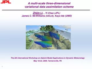
A multi-scale three-dimensional variational data assimilation scheme
A multi-scale three-dimensional variational data assimilation scheme. Zhijin Li , , Yi Chao (JPL) James C. McWilliams (UCLA), Kayo Ide (UMD). The 8th International Workshop on Adjoint Model Applications in Dynamic Meteorology May 18-22, 2009, Tannersville, PA. Outline. Motivations

A multi-scale three-dimensional variational data assimilation scheme
E N D
Presentation Transcript
A multi-scale three-dimensional variational data assimilation scheme Zhijin Li, , Yi Chao (JPL) James C. McWilliams (UCLA), Kayo Ide (UMD) The 8th International Workshop on Adjoint Model Applications in Dynamic Meteorology May 18-22, 2009, Tannersville, PA
Outline • Motivations • A multi-scale three-dimensional variational data assimilation (MS-3DVAR) scheme • Applications and evaluations • Summary
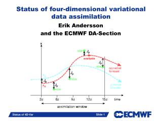
3-day forecast 6-hour forecast xf 6-hour assimilation cycle xa Initial condition Time Aug.2 00Z Aug.1 18Z Aug.1 06Z Aug.1 12Z Aug.1 00Z Data Assimilation and Forecast Cycle Time scales comparable with those of the atmosphere
Observations and Data assimilation • T/S profiles from gliders • Ship CTD profiles • Aircraft SSTs • AUV sections • HF radar velocities AOSN-II
Performance of ROMS3DVAR: AOSN-II, August 2003 Comparison of Glider-Derived Currents (vertically integrated current) SALT(PSU) Black: SIO glider; Red: ROMS TEMP(C) Glider temperature/salinity profiles (Chao et al., 2009, DSR)
Challenge: An Example with SCCOOS Model domain, the resolution of 1km
Southern California Coastal Ocean Observing System (SCCOOS) Aug 2008, simulation without DA SIO Glider Tracks Challenge: How to assimilate sparse vertical profiles along with high resolution observations for a very high resolution model
Variational methods (3Dvar/4Dvar): • prescribed B • optimization algorithm Sequential methods (Kalman filter/smoother) • dynamically evolved B • analytical solution Data Assimilation Formulation
RMSE diagonal matrix C: Correlation matrix Error Covariance and correlations Correlations are the vehicle for spreading out information of observations Correlation scales are about 15-30km
Forecast Error Covariance B:Single Observation Experiment (increment) One single observation of SSH
Southern California Coastal Ocean Observing System (SCCOOS) SIO Glider Tracks Motivation: assimilating sparse vertical profiles along with high resolution observations for a very high resolution model
Background Observation Prerequisites Multi-scale DA Multi-Scale Data Assimilation: Concept SCCOOS Glider Tracks (Boer, 1983, MWR)
Multi-Scale Data Assimilation: Scheme Low Resolution (LR) SCCOOS Glider Tracks Sparse Obs High Resolution (HR) High resolution HF radar High Resolution Obs
Work Flowchart of MS-3DVAR Smoothed Satellite SST/SSH Glider/Argo/Mooring HF Radar LR-3DVAR HR-3DVAR End Smoothed Forecast Increment Start
Glider Observations vs Analyses Aug 2008
CALCOFI Observations (not assimilated) Aug 14-30, 2008
Monthly Means Aug, 2008
Analysis vs HF Radar Observations Taylor diagram (Taylor, 2001, JGR)
Surface Currents Forecasts vs Analyses
Summary • A multi-scale 3DVAR (MS-3DVAR) scheme has been formulated and developed. • It has been implemented in support of SCCOOS and AOOS-PWS. • The scheme has demonstrated the capability of assimilating sparse and high resolutions observations simultaneously, effectively and reliably.
Alaska Ocean Observing System -Prince William Sound:AOOS-PWS 3 nested levels: L0 / L1 / L2. Resolution : 10km / 3.6km / 1.2 km (L2 : Prince William Sound)
Oil Spill: 1989 Exxon Tanker Wreck Prince William Sound, Alaska March 24, 1989 From USGS Today
Decomposition of Large and Small Scalesand Estimation of Error Covariance • Generate perturbations: difference between 24h and 48h forecasts, valid at the same time. • Decompose perturbations Large scales: smoothed fields, with weight of where L=25km, which is the decorrelation length scale from Russ’s estimation Small scales: the residuals
Observational Errors: Representativeness Errors • Large scale observations: T/S vertical profiles from SIO, mooring and Argo • Observational errors at the depth of z: • Tentative values: briefly and empirically estimated from the RMS profile of the small scale components For temperature For salinity CALCOFI Section
Future Coastal Observing System (National Research Council, 2003) • Buoy and glider profiles are sparse, with distances between profiles larger than decorrelation scales • Radar and satellite measurements may have very high resolutions, as high as the model resolution
Surface Tidal Current Comparison (M2) Length of Major Axis (cm/s) Corr. RMS Mean Sept. 0.43 3.6 6.6 Oct. 0.44 3.8 6.6 Nov. 0.51 3.7 6.3
A There-Dimensional Variational Data Assimilation (3DVAR) • Real-time capability • Implementation with sophisticated and high resolution model configurations • Flexibility to assimilate various observation simultaneously • Development for more advanced scheme (Li et al., 2006, MWR; Li et al., 2008, JGR, Li et al., 2008, JAOT)