Capacitively Coupled Resistivity Survey of the Sea Ice Near Barrow, Alaska Dr. Rhett Herman, James Inman

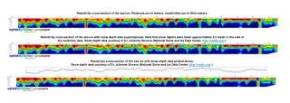
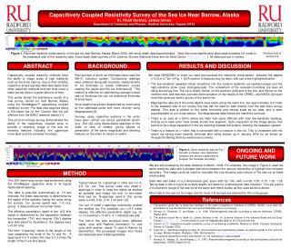
1. Capacitively Coupled Resistivity Survey of the Sea Ice Near Barrow, Alaska Dr. Rhett Herman, James Inman Department of Chemistry and Physics , Radford University, Virginia 24142 Figure 1. Electrical resistivity cross-section of the sea ice near Barrow, Alaska, March 2006, with snow depth data superimposed. Note that snow depths were taken approximately 2/3 meter to the (seaward) side of the resistivity data. Snow depth data courtesy of Dr. Julienne Stroeve (National Snow and Ice Data Center, http://nsidc.org/ ). All distances are in meters. Northern end of survey line ABSTRACT BACKGROUND RESULTS AND DISCUSSION Capacitively coupled resistivity methods have the ability to image areas of high resistivity such as the arctic sea ice. Due to their mobility, capacitive arrays typically take data faster than other resistivity methods and can thus cover a wider survey area in a given amount of time. This poster shows the preliminary results of a new survey carried out near Barrow, Alaskausing the OhmMapper™ capacitively coupled resistivity survey. The data was acquired along a 300-meter line on the Chukchi Sea ice just offshore from the BASC research station.[1] This proof-of-concept survey demonstrates the ability of the capacitively coupled array to provide a resistivity image of the sea ice showing features including the uppermost snow layer and the ice/water boundary. Past surveys of arctic ice thickness have used the EM-31 induction system. Conductivity readings were obtained along with borehole measurements of ice thickness to create calibration curves relating the signal and the ice thickness.[2] This method is effective for determining average overall sea ice thickness but can not determine thickness of snow layer. Snow depths have been determined by hand using at first calibrated poles and more recently using Magnaprobes [3]. Surveys using capacitive systems in the arctic have been carried out across permafrost terrain (e.g., Ref. [4]) using dipole-dipole spacings on the order of tens of meters, giving depths of penetration of the same magnitude and showing features on the order of meters in extent. • We used RES2DINV to invert our data and produce the resistivity cross-section between the depths z~0.21m-2.72m in Fig. 1. [6] A number of features may be seen, with just a few highlighted below. • The low-resistivity seawater (blue) transitions into the medium-resistivity ice (yellow/orange) and the high-resistivity snow cover (orange/purple). The undulations of the ice/water boundary are seen all along the survey line. The ice is clearly thicker on the southern (left) end of the line, and thinner on the northern end, and matches a private communication of the results of the CRREL- and NSIDC-led team from their previous week’s survey of the same line. • Magnaprobe data [3] of the snow depths were taken along the same line, but approximately 2/3 meter to the seaward side of our survey line (we did not want to walk directly over the test line’s survey stakes). This data is plotted on the same horizontal and vertical scale as our data, and is seen superimposed on our cross-section. The Magnaprobe data follows the resistivity contours. • There is an area at x~241m where we often had some difficulty with very low-resistivity readings, forcing us to walk even more slowly across this segment. Upon inspection of the image above, this seems to be a large separation in the ice reaching towards the surface, allowing the seawater upward. • There is a feature at x~148m that is consistent with a fracture in the ice. This is consistent with the area’s ice having been recently reformed after being broken up in January 2006 by ice forced up through the Bering Strait by wind/ocean currents. ONGOING AND FUTURE WORK Figure 2. Same resistivity data as Fig. 1 but with a sharper color distinction between the various resistivities to sharpen the ice/water boundary. We are still processing the data obtained in March, 2006. For example, the image in Figure 2 used the same resistivity data with a sharper distinction between the various resistivities to highlight the ice/water boundary. This image could be used to calculate the true structure and volume of the sea ice at these small scales. Data was also taken in a 2-dimensional grid, size=100m by 10m, with n=0.25, 0.50, 0.75, 1.00, 1.25. Taking data in this 2-d grid at multiple depths will allow for 3-dimensional data inversion. This will yield a 3-d volumetric image of the sea ice at the same sub-meter scales as the cross-sections above. More trips to the sea ice for longer and for more 3-D surveys are planned for the coming year. METHOD This 300-meter-long survey was performed using the OhmMapper capacitive array in its typical dipole-dipole spacing. The data is acquired automatically at 1.0 sec intervals; the linear data density is determined by the speed of the operator towing the array along the surface. Our survey speed was ~1/3 m/s, giving ~3 data points per horizontal meter. The effective penetration depth of the 16.5 kHz signal is determined by the separation between the transmitter (“Tx”) and receiver (“Rx”) dipoles (see side panel for illustration). Our dipoles were L=5.0m long. The term “n-spacing” refers to the length of the rope separating the ends of the Tx and Rx . A spacing of n=1.0 means the rope is 1.0 times the length of the Tx (or Rx) dipole. Typical values for n-spacings in other are n=1.0, 2.0, 3.0, etc. This survey used very small n-spacings in order to keep the signal as shallow as possible and image the one- to two-meter thick sea ice. N-spacings used in this survey were n=0.25, 0.50, 0.75, 1.00 and 1.25. Our set of small n-spacings extensively probed the shallow ice. For example, our L=5.0 meter dipoles, the effective penetration depth e.g. for n=1.0 would be z~0.42*L~2.1 meters [Loke pdf]. The 300-m line was surveyed twice (different days), once with Radford University’s Tx, and once with another, newer Tx sent to Barrow by Geometrics. The processed images from these two data sets were indistinguishable. References • The authors would like to thank the members of the team consisting of members of CRREL, NSIDC, et al team for permission to use the test line they surveyed immediately prior to our survey. • Kovacs, A., Diemand, D., and Bayer, J. Jr., 1996, Electromagnetic induction sounding of sea ice thickness. CRREL Report 96-6. • The authors would like to thank Dr. Juliene Stroeve of the Dr. Julienne Stroeve of the National Snow and Ice Data Center (http://nsidc.org/ ) for permission to use her Magnaprobe data on the Chukchi test line. • Calvert, H. T., Capacitive-coupled resistivity survey of ice-bearing sediments, Mackenzie Delta, Canada. Geological Survey of Canada, 2002. • Loke, M. L., Electrical imaging surveys for environmental and engineering studies—a practical guide to 2-D and 3-D surveys, Minden Heights, Malaysia, 1999. Distributed by http://www.geoelectrical.com. • The authors would like to thank Geometrics, Inc. for assistance in data analysis. • Kovacs, A., Valleau, N., and Holladay, J. S., 1987, Airborne electromagnetic sounding of sea ice thickness and sub-ice bathymetry. CRREL Report 87-23.