Analyzing categorical data
This guide explores the analysis of categorical data, defined by non-continuous (discrete) values representing distinct categories such as binary options ("yes/no", "high/low") and multi-category variables ("agree/neutral/disagree"). It presents various methods for comparing groups, including constructing confidence intervals, performing z-tests, and using chi-square tests to assess the differences in proportions. The content emphasizes the significance of confidence intervals and probability values when interpreting categorical data outcomes and testing hypotheses effectively.

Analyzing categorical data
E N D
Presentation Transcript
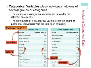
Categorical data • Non-continuous (discrete values) • Categories such as: • “high” or “low” • Yes / no • Graduate / non-graduate • College vs. non-college These are binary variables • Or multiple categories • High/medium/low • Agree/neutral/disagree • Elementary/middle/high school • Public / private school Sometimes the categorical variables are just categories (sometimes call “nominal”). Other times they may represent some order (ordinal).
Approaches for comparing groupsWhen we have categorical data Parallel to our strategies for comparing means • Construct separate confidence intervals • Do they overlap? • Construct a confidence interval on the difference • Does the CI include zero? • A z-test on the difference between the proportions • Very similar to a t-test for the means • The chi-square test (NHST) • Is the probability value less than .05 (our alpha level or significance level)? Options 1,2 and 3 are parallels to our approaches for comparing means. These all work fine for two groups. Option 4 is something new. It works for two groups, or more than two groups. So it is very versatile.
CI approachDo they overlap? • Example 1: 95% CI: Null hypothesis: The proportions in the populations are equal. H0: Pa= Pb or H0: pa = pb Conclusion: The CIs overlap. We cannot reject Ho. We cannot conclude that the population proportions are different.
CI for the difference is the pooled proportion (using the sample sizes as weights) Here the pooled p (p-hat) is .68 95% CI: .10 ± .11 Or: [ -0.01 , .21 ] Conclusion: The CI includes zero. We cannot reject Ho. We cannot conclude that the population proportions are different.
A z-test for the difference between the sample proportions This is very parallel to a t-test on the means. = In this example, we get z = 1.75 p = .04 (1 tailed) p = .08 (2-tailed) Conclusion: The probability value is not less than 0.05. We cannot reject Ho. We cannot conclude that the population proportions are different.
Example 2Three approaches Next: Let’s use a chi-square test