Enhancing Data Fitting Techniques Using Scaling, Orthogonalization, and Principal Component Analysis
This guide covers the application of advanced data fitting techniques, including scaling profiles to match data dimensions and constructing orthogonal basis functions via methods such as the Gram-Schmidt process. We delve into concepts of basis vectors in data space, analyzing the impact of length scales and contour behavior in χ² fitting. By applying techniques like Principal Component Analysis (PCA) and periodogram analysis for sinusoidal signals, we demonstrate how to optimize fits amid varying error scales. Explore the nuances of fitting polynomials and sinusoidal functions effectively.

Enhancing Data Fitting Techniques Using Scaling, Orthogonalization, and Principal Component Analysis
E N D
Presentation Transcript
x2 x2 x1 e2 x1 e1 Example
Scaling a profile to fit data • Using the notation we’ve just learned, • So what basis vectors correspond to ? • Answer: • i.e. i is the unit of distance on the ith axis of data space!
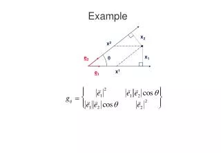
Length scales • In the orthogonal system we used for profile fitting: • Dot product of 2 basis vectors: • i.e. the basis vectors are orthogonal, but not unit length. • Need to stretch axis i by factor i and define new basis vectors b:
contours are ellipses x2 x e2 e1 x1 ellipses become circles • Old basis vectors: • Stretched basis vectors: b2 contours are circles x2 /2 x b1 b2 b1 x1 /1
He/H O/H x y=ax+b y Example: primordial helium abundance • Fitting a line to data with error bars in both X and Y: • If x≠y, get misleading point of closest approach • Horizontal stretch by factor y/x: x y=a’x’+b R y
Defining with errors in both X and Y • Hence determine minimum distance R: • Hence:
Constructing orthogonal basis functions • First way: diagonalize Hessian matrix. • Quadratic approximation to surface: • Orthogonal basis vectors are the eigenvectors of Hij along the principal axes of the contours. • Sometimes called “Principal Component Analysis” (PCA), also related to singular-value decomposition (see Press et al).
v2 v1 v3 v1 e1 v2 v2’ e1 Gram-Schmidt Orthogonalization – 1 • Second way: the Gram-Schmidt process. • 1. Start with N vectors Vi , i=1,...N. They must be independent, i.e. no two of them parallel. • 2. Normalize vector 1: • 3. Make v2’ perpendicular to e1: • i.e. subtract component of v2 in direction of e1 • 4. Normalize v2’ : v2’ e1 e2
v3’ v3 e1 v3’ v3” e2 v3” e3 Gram-Schmidt Orthogonalization – 2 • 5. Make v3’ perpendicular to e1: • 6. Make v3” perpendicular to e2: • Note: v3” is perpendicular to e1 AND e2. • 7. Normalize v3”: • ...and so on, making v4 perpendicular to e1, e2, e3 and normalising to get e4 • Repeat for all vectors up to vN to get ortho-normal basis e1, e2, ..., eN
Differences between successive fits • Fit: A + B x + C x2 • A, B, C are not independent • 1, x, x2 are not orthogonal • If Pk(x) is a polynomial of degree k fitted to the data, then fit: • AP0(x) + B[P1(x) - P0(x)] + C [P2(x) - P1(x)] • A, B, C are independent • the functions Pk(x) - Pk-1(x) are orthogonal
S A C Wrong : bad , small A S C Phase 0 1 Periodic signals • To search a time series of data for a sinusoidal oscillation of unknown frequency : • “Fold” data on trial period P • Fit a function of the form: Programming hint: Use phi=atan2(–S,C) if you care about which quadrant ends up in! Correct : good , large A S Phase 0 1 C
S S C C Periodograms • Repeat for a large number of values • Plot A() vs to get a periodogram: A()
Fitting a sinusoid to data • Data: ti, xi ± i, i=1,...N • Model: • Parameters: X0, C, S, • Model is linear in X0, C, S and nonlinear in • Use an iterative fit to linear parameters at a sequence of fixed trial .
Iterate to convergence: • Error bars: