Review 2: Illumination, Shading, Texturing and Anti-aliasing

1. Review 2: Illumination, Shading, Texturing and Anti-aliasing Jian Huang, CS594, Spring 2002

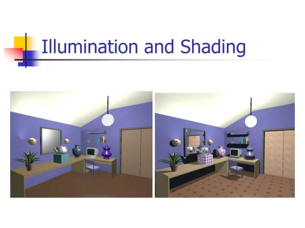
2. Illumination Vs. Shading • Illumination (lighting) model: determine the color of a surface point by simulating some light attributes. • Shading model: applies the illumination models at a set of points and colors the whole image.

3. Local illumination • Only consider the light, the observer position, and the object material properties

4. Basic Illumination Model • Simple and fast method for calculating surface intensity at a given point • Lighting calculating are based on: • The background lighting conditions • The light source specification: color, position • Optical properties of surfaces: • Glossy OR matte • Opaque OR transparent (control refection and absorption)

5. Ambient light (background light) • The light that is the result from the light reflecting off other surfaces in the environment • A general level of brightness for a scene that is independent of the light positions or surface directions -> ambient light • Has no direction • Each light source has an ambient light contribution, Ia • For a given surface, we can specify how much ambient light the surface can reflect using an ambient reflection coefficient : Ka (0 < Ka < 1)

6. Ambient Light • So the amount of light that the surface reflect is therefore Iamb = Ka * Ia

7. Diffuse Light • The illumination that a surface receives from a light source and reflects equally in all directions • This type of reflection is called Lambertian Reflection (thus, Lambertian surfaces) • The brightness of the surface is indepenent of the observer position (since the light is reflected in all direction equally)

8. Lambert’s Law • How much light the surface receives from a light source depends on the angle between its angle and the vector from the surface point to the light (light vector) • Lambert’s law: the radiant energy ’Id’ from a small surface da for a given light source is: Id = IL * cos(q) IL : the intensity of the light source • is the angle between the surface normal (N) and light vector (L)

9. The Diffuse Component • Surface’s material property: assuming that the surface can reflect Kd (0<Kd<1), diffuse reflection coefficient) amount of diffuse light: Idiff = Kd * IL * cos(q) If N and L are normalized, cos(q) = N*L Idiff = Kd * IL * (N*L) • The total diffuse reflection = ambient + diffuse Idiff = Ka * Ia + Kd * IL * (N*L)

10. Examples Sphere diffusely lighted from various angles !

11. Specular Light • These are the bright spots on objects (such as polished metal, apple ...) • Light reflected from the surface unequally to all directions. • The result of near total reflection of the incident light in a concentrated region around the specular reflection angle

12. Phong’s Model for Specular • How much reflection light you can see depends on where you are

13. Phong Illumination Curves Specular exponents are much larger than 1; Values of 100 are not uncommon. : glossiness, rate of falloff

14. Specular Highlights • Shiny surfaces change appearance when viewpoint is changed • Specularities are caused by microscopically smooth surfaces. • A mirror is a perfect specular reflector

15. Phong Illumination Moving Light Change n

16. Putting It All Together • Single Light (white light source)

17. Flat Shading

18. Smooth Shading • Need to have per-vertex normals • Gouraud Shading • Interpolate color across triangles • Fast, supported by most of the graphics accelerator cards • Phong Shading • Interpolate normals across triangles • More accurate, but slow. Not widely supported by hardware

19. Gouraud Shading • Normals are computed at the polygon vertices • If we only have per-face normals, the normal at each vertex is the average of the normals of its adjacent faces • Intensity interpolation: linearly interpolate the pixel intensity (color) across a polygon surface

20. Gouraud Shading

21. Phong Shading Model • Gouraud shading does not properly handle specular highlights, specially when the n parameter is large (small highlight). • Reason: colors are interpolated. • Solution: (Phong Shading Model) • 1. Compute averaged normal at vertices. • 2. Interpolate normals along edges and scan-lines. (component by component) • 3. Compute per-pixel illumination.

22. Phong Shading

23. What Dreams May Come

24. How to efficiently add graphics detail? • Solution - (its really a cheat!!) • How? MAP surface detail from a predefined (easy to model) table (“texture”) to a simple polygon

25. Texture Mapping • Problem #1 • Fitting a square peg in a round hole • We deal with non-linear transformations • Which parts map where?

26. Texture Mapping • Problem #2 • Mapping from a pixel to a “texel” • Aliasing is a huge problem!

27. What is a Texture? • Given the (texture/image index) (u,v), want: • F(u,v) ==> a continuous reconstruction • = { R(u,v), G(u,v), B(u,v) } • = { I(u,v) } • = { index(u,v) } • = { alpha(u,v) } • = { normals(u,v) } • = { surface_height(u,v) } • = ...

28. RGB Textures • Places an image on the object • “Typical” texture mapping

29. Opacity Textures • A binary mask, really redefines the geometry.

30. Bump Mapping • This modifies the surface normals. • More on this later.

31. Displacement Mapping • Modifies the surface position in the direction of the surface normal.

32. Texture and Texel • Each pixel in a texture map is called a Texel • Each Texel is associated with a (u,v) 2D texture coordinate • The range of u, v is [0.0,1.0]

33. (u,v) tuple • For any (u,v) in the range of (0-1, 0-1), we can find the corresponding value in the texture using some interpolation

34. Two-Stage Mapping • Model the mapping: (x,y,z) -> (u,v) • Do the mapping

35. Image space scan For each y For each x compute u(x,y) and v(x,y) copy texture(u,v) to image(x,y) • Samples the warped texture at the appropriate image pixels. • inverse mapping

36. Image space scan • Problems: • Finding the inverse mapping • Use one of the analytical mappings • Bi-linear or triangle inverse mapping • May miss parts of the texture map Texture Image

37. Inverse Mapping • Need to transform back to world space to do the interpolation • Orientation in 3D image space • Foreshortening (.8,1) (.5,1) (.5,.7) (.1,.6) (.6,.2)

38. Texture space scan For each v For each u compute x(u,v) and y(u,v) copy texture(u,v) to image(x,y) • Places each texture sample to the mapped image pixel. • Forward mapping

39. Texture space scan • Problems: • May not fill image • Forward mapping needed Image Texture

40. Texture Mapping • Mapping to a 3D Plane • Simple Affine transformation • rotate • scale • translate y z v x u

41. Texture Mapping • Mapping to a Cylinder • Rotate, translate and scale in the uv-plane • u -> q • v -> z • x = r cos(q), y = r sin(q) v u

42. Texture Mapping • Mapping to Sphere • Impossible!!!! • Severe distortion at the poles • u -> q • v -> f • x = r sin(q) cos(f) • y = r sin(q) sin(f) • z = r cos(q)

43. Sampling • What we have in computer graphics is a point sampling of our scene, or: • I(x) = f(x)•ST(x) • What we would like is more of an integration across the pixel (or larger area): • I(x) = f(x) h(x) • What should h(x) be?

44. Sampling Theorem • The Shannon Sampling Theorem A band-limited signal f(x), with a cutoff frequency of l, that is sampled with a sampling spacing of T may be perfectly reconstructed from the discrete values f[nT] by convolution with the sinc(x) function, provided: l is called the Nyquist limit.

45. Sampling and Anti-aliasing • If don’t have Nyquist rate, then aliasing artifacts.

46. Two possible solutions • So far we just mapped one point, results in bad aliasing (resampling problems) • Two possible solutions: • Super-sampling: not very good (slow!) • Low-pass filtering: popular approaches – mipmaps, SAT

47. Quality considerations • Pixel area maps to “weird” (warped) shape in texture space v ys pixel xs u

48. Quality considerations • We need to: • Calculate (or approximate) the integral of the texture function under this area • Approximate: • Convolve with a wide filter around the center of this area • Calculate the integral for a similar (but simpler) area.

49. Quality considerations • the area is typically approxiated by a rectangular region (found to be good enough for most applications) • filter is typically a box/averaging filter - other possibilities • how can we pre-compute this?

50. v ys pixel xs u Summed Area Table (SAT) • Determining the rectangle: • Find bounding box and calculate its aspect ratio