Download
1 / 11
160 likes | 621 Vues
Se busca la solución de un problema de la forma Ax = b o Ax – b =0, donde A es una matriz cuadrada formada por los coeficientes de un sistema de ecuaciones lineales de la forma, y x las variables del sistema y b las soluciones

E N D
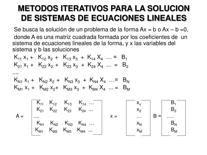
Se busca la solución de un problema de la forma Ax = b o Ax – b =0, donde A es una matriz cuadrada formada por los coeficientes de un sistema de ecuaciones lineales de la forma, y x las variables del sistema y b las soluciones K11 x1 + K12 x2 + K13 x3 + K14 X4 … = B1 K21 x1 + K22 x2 + K23 x3 + K24 X4 ... = B2 .... KN1 x1 + KN2 x2 + KN3 x3 + KN4 X4 …= BN KM1 x1 + KM2 x2+ KM3 x3 + KM4 X4 ... = BM K11 K12 K13 K14 … xx B1 K21 K22 K23 K24 ... x2 B2 A = .... x = … B = …. KN1 KN2 KN3 KN4 … xN BN KM1 KM2 KM3 KM4 ... xM BM METODOS ITERATIVOS PARA LA SOLUCION DE SISTEMAS DE ECUACIONES LINEALES
METODOS USADOS EJEMPLO Sea el siguiente sistema de ecuaciones lineales resolver por el método de Jacobi y Gauss-Seidel 10x1 - x2 + 2x3 = 6 -x1 + 11x2 - x3 + 3x4 = 25 2x1 - x2 + 10x3 - x4 = -11 - 3x2 - x3 + 8x4 = 15 Solucionando el problema por Jacobi:
Y se obtiene el siguiente archivo de programación en SCILAB function [x]= jacobi(x0,tol) // Nombre del Archivo: jacobi.sci // // Programa para resolver el siguiente sistema de // ecuaciones lineales por el metodo de Jacobi : // // 10x1 - x2 + 2x3 = 6 // -x1 + 11x2 - x3 + 3x4 = 25 // 2x1 - x2 + 10x3 - x4 = -11 // - 3x2 - x3 + 8x4 = 15 // // Utilizacion: x = jacobi(x0,tol) // Input: x0= Punto inicial de iteracion // tol= tolerancia del error // // Output: x=Aproximacion de solucion del // sistema de ecuaciones //
Xant=[x0(1);x0(2);x0(3);x0(4);1]; T=[0,1/10,-2/10,0,6/10;1/11,0,1/11,-3/11,25/11;-2/10,1/10,0,1/10,-11/10; 0,-3/8,1/8,0,15/8]; Xnew=[9999;9999;9999;9999;9999]; n=0; while (norm(Xnew-Xant)/norm(Xnew)) > tol if n>=1 then Xant=Xnew;end; Xnew=T*Xant, Xnew=[Xnew;1] n=n+1, end; x=Xnew(1:4) disp(n,'Numero de iteraciones ')
Los resultados obtenidos son los siguientes: -->getf('C:\jacobi.sci');disp('getf done'); getf done -->x0=[0,0,0,0]; -->tol=10^(-5); -->x=jacobi(x0,tol) Numero de iteraciones 15. ans = ! .9999982 ! ! 2.0000029 ! ! - 1.0000023 ! ! 1.0000034 !
Si disminuimos la tolerancia o error (tol), obtendremos un valor mas exacto -->x0=[0,0,0,0]; -->tol=10^(-9); -->x=jacobi(x0,tol) Numero de iteraciones 26. x = ! 1. ! ! 2. ! ! - 1. ! ! 1. ! Como vemos hemos obtenido el valor exacto de la solución del sistema de ecuaciones 4x4, en 26 iteraciones,
Para el método de Gauss-Seidel, se tiene la siguiente función: function [x]=gauss(x0,tol) // Nombre del Archivo: gaussseidel.sci // // Programa para resolver el siguiente sistema de // ecuaciones lineales por el metodo de Gauss-Seidel: // // 10x1 - x2 + 2x3 = 6 // -x1 + 11x2 - x3 + 3x4 = 25 // 2x1 - x2 + 10x3 - x4 = -11 // - 3x2 - x3 + 8x4 = 15 // // Utilizacion: x = gauss(x0,tol) // Input: x0= Punto inicial de iteracion // tol= tolerancia del error // // Output: x=Aproximacion de solucion del // sistema de ecuaciones //
Xant=[x0(1);x0(2);x0(3);x0(4);1]; T=[0,1/10,-2/10,0,6/10;1/11,0,1/11,-3/11,25/11;-2/10,1/10,0,1/10,-11/10; 0,-3/8,1/8,0,15/8]; Xnew=[9999;9999;9999;9999;9999]; n=0; while (norm(Xnew - Xant)/norm(Xnew)) > tol Xnew=Xant; Xant(1,1)=T(1,:)*Xant; Xant(2,1)=T(2,:)*Xant; Xant(3,1)=T(3,:)*Xant; Xant(4,1)=T(4,:)*Xant; n=n+1; end; x=Xant(1:4); disp(n,'Numero de iteraciones')
Del cual se obtienen los siguientes resultados: -->getf('C:\gaussseidel.sci');disp('getf done'); getf done -->x0=[0,0,0,0]; -->tol=10^(-5); -->x=gauss(x0,tol) Numero de iteraciones 7. x = ! 1.0000007 ! ! 2. ! ! - 1.0000002 ! ! 1.0000000 !
Disminuyendo también la tolerancia se obtiene: -->x0=[0,0,0,0]; -->tol=10^(-9); -->x=gauss(x0,tol) Numero de iteraciones 10. x = ! 1. ! ! 2. ! ! - 1. ! ! 1. ! Como Podemos ver se logra alcanzar la solución exacta del sistema de ecuaciones lineales 4x4 , en 10 iteraciones
Como podemos ver Gauss-Seidel convergió a la solución exacta mucho mas rápido que Jacobi, casi en un tercio del tiempo empleado por este. • Además si comparamos de igual modo las soluciones aproximadas, vemos que Gauss también convergió más rápido que Jacobi, e incluso con un error algo menor.