Inference on a Single Mean
Inference on a Single Mean. Use Calculation from Sample to Estimate Population Parameter. (select). Population. Sample. (calculate). (describes). (estimate). Parameter. Statistic. Use Calculation from Sample to Estimate Population Parameter. (select). Population. Sample. (calculate).

Inference on a Single Mean
E N D
Presentation Transcript
Inference on a Single Mean G. Baker, Department of Statistics University of South Carolina
Use Calculation from Sample to Estimate Population Parameter (select) Population Sample (calculate) (describes) (estimate) Parameter Statistic G. Baker, Department of Statistics University of South Carolina; Slide 2
Use Calculation from Sample to Estimate Population Parameter (select) Population Sample (calculate) (describes) (estimate) Parameter Statistic G. Baker, Department of Statistics University of South Carolina; Slide 3
Describes a sample. Always known Changes upon repeated sampling. Examples: Describes a population. Usually unknown Is fixed Examples: Statistic Parameter G. Baker, Department of Statistics University of South Carolina; Slide 4
A Statistic is a Random Variable • Upon repeated sampling of the same population, the value of a statistic changes variable. • While we don’t know what the next value will be, we do know the overall pattern over many, many samplings random. • The distribution of possible values of a statistic for repeated samples of the same size from a population is called the sampling distribution of the statistic. G. Baker, Department of Statistics University of South Carolina; Slide 5
Sampling Distribution of • If a random sample of size n is taken from a normal population having mean μyand variance σy2, then is a random variable which is also normally distributed with mean μyand variance σy2/n . G. Baker, Department of Statistics University of South Carolina; Slide 6
Sampling Distribution of n(100,5) n(100,1.58) n(100,3.54) n(100,1) G. Baker, Department of Statistics University of South Carolina; Slide 7
Light Bulbs • The life of a light bulb is normally distributed with a mean of 2000 hours and standard deviation of 300 hours. • What is the probability that a randomly chosen light bulb will have a life of less than 1700 hours? • What is the probability that the mean life of three randomly chosen light bulbs will be less than 1700 hours? G. Baker, Department of Statistics University of South Carolina; Slide 8
Why Averages Instead of Single Readings? • Suppose we are manufacturing light bulbs. The life of these bulbs has historically followed a normal distribution with a mean of 2000 hours and standard deviation of 300 hours. • We change the filament material and unknown to us the average life of the bulbs decreases to 1500 hours. (We will assume that the distribution remains normal with a standard deviation of 300 hours.) • If we randomly sample 1 bulb, will we realize that the average life has decrease? What if we sample 3 bulbs? 9 bulbs? G. Baker, Department of Statistics University of South Carolina; Slide 9
Why Averages Instead of Single Readings? σ = 300 μ = 1500 μ = 2000 Single Readings Y < 1400 would signal shift G. Baker, Department of Statistics University of South Carolina; Slide 10
Why Averages Instead of Single Readings? σ = 173 μ = 1500 μ = 2000 Averages of n = 3 Y < 1654 would signal shift G. Baker, Department of Statistics University of South Carolina; Slide 11
Why Averages Instead of Single Readings? µ = 1500 µ = 2000 σ = 100 µ = 1500 μ = 1500 µ = 2000 μ = 2000 Averages of n = 9 Y < 1800 would signal shift G. Baker, Department of Statistics University of South Carolina; Slide 12
What if the original distribution is not normal? Consider the roll of a fair die: G. Baker, Department of Statistics University of South Carolina; Slide 13
Suppose the single measurements are not normally Distributed. • Let Y = time to fail of a light bulb in constant failure rate mode • Y is exponentially distributed with λ = 0.0005 = 1/2000 0.0005 G. Baker, Department of Statistics University of South Carolina; Slide 14
Single measurements Averages of 2 measurements Averages of 4 measurements Source: Lawrence L. Lapin, Statistics in Modern Business Decisions, 6th ed., 1993, Dryden Press, Ft. Worth, Texas. Averages of 25 measurements G. Baker, Department of Statistics University of South Carolina; Slide 15
As n increases, what happens to the variance? n=1 n=2 • Variance increases. • Variance decreases. • Variance remains the same. n=4 n=25 G. Baker, Department of Statistics University of South Carolina; Slide 16
n = 1 n = 2 n = 4 n = 25 G. Baker, Department of Statistics University of South Carolina; Slide 17
Central Limit Theorem • If n is sufficiently large, the sample means of random samples from a population with mean μ and standard deviation σ are approximately normally distributed with mean μ and standard deviation . G. Baker, Department of Statistics University of South Carolina; Slide 18
Random Behavior of Means Summary • If Y is distributed n(μ, σ), then is distributed n(μ, ). • If Y is distributed non-n(μ, σ), then is distributed approximately n(μ, ). G. Baker, Department of Statistics University of South Carolina; Slide 19
If We Can Consider to be Normal … • Recall: If Y is distributed normally with mean μ and standard deviation σ, then • So if is distributed normally with mean μ and standard deviation , then G. Baker, Department of Statistics University of South Carolina; Slide 20
If the time between industrial accidents follows an exponential distribution with an average of 700 days, what is the probability that the average time between 49 pairs of accidents will be greater than 900 days? G. Baker, Department of Statistics University of South Carolina; Slide 21
XYZ Bottling Company claims that the distribution of fill on it’s 16 oz bottles averages 16.2 ounces with a standard deviation of 0.1 oz. We randomly sample 36 bottles and get y = 16.15. If we assume a standard deviation of 0.1 oz, do we believe XYZ’s claim of averaging 16.2 ounces? G. Baker, Department of Statistics University of South Carolina; Slide 22
Up Until Now We have been Assuming that We Knew the True Standard Deviation (σ), But Let’s Face Facts … • When we use s to estimate σ, then the calculated value follows a t-distribution with n-1 degrees of freedom. Note: we must be able to assume that we are sampling from a normal population. G. Baker, Department of Statistics University of South Carolina; Slide 23
Let’s take another look at XYZ Bottling Company. If we assume that fill on the individual bottles follows a normal distribution, does the following data support the claim of an average fill of 16.2 oz? 16.1 16.0 16.3 16.2 16.1 G. Baker, Department of Statistics University of South Carolina; Slide 24
In Summary • When we know σ: • When we estimate σ with s: We assume we are sampling from a normal population. G. Baker, Department of Statistics University of South Carolina; Slide 25
Relationship Between Z and t Distributions Z tdf=3 tdf=1 G. Baker, Department of Statistics University of South Carolina; Slide 26
Internal Combustion Engine • The nominal power produced by a student-designed internal combustion engine should be 100 hp. The student team that designed the engine conducted 10 tests to determine the actual power. The data follow: 98, 101, 102, 97, 101, 98, 100, 92, 98, 100 Assume data came from a normal distribution. G. Baker, Department of Statistics University of South Carolina; Slide 27
Internal Combustion Engine Summary Data: What is the probability of getting a sample mean of 98.7 hp or less if the true mean is 100 hp? G. Baker, Department of Statistics University of South Carolina; Slide 28
Internal Combustion Engine 0.0949 What did we assume when doing this analysis? Are you comfortable with the assumption? G. Baker, Department of Statistics University of South Carolina; Slide 29
Can We Assume Sampling from a Normal Population? • If data are from a normal population, there is a linear relationship between the data and their corresponding Z values. If we plot y on the vertical axis and z on the horizontal axis, the y intercept estimates μ and the slope estimates σ. G. Baker, Department of Statistics University of South Carolina; Slide 30
How to Calculate Corresponding Z-Values • Order data • Estimate percent of population below each data point. • Look up Z-Value that has Pi proportion of distribution below it. where i is a data point’s position in the ordered set and n is the number of data points in the set. G. Baker, Department of Statistics University of South Carolina; Slide 31
Normal Probability (QQ) Plot Z Pi yi i -1.15 .125 2 1 -0.32 .375 4 2 +0.32 .625 7 3 +1.15 .875 10 4 2 4 7 10 Data set: G. Baker, Department of Statistics University of South Carolina; Slide 32
Normal Probability (QQ) Plot This data is a random sample from a n(10,2) population. G. Baker, Department of Statistics University of South Carolina; Slide 33
Normal Probability (QQ) Plot G. Baker, Department of Statistics University of South Carolina; Slide 34
Estimation of the Mean G. Baker, Department of Statistics University of South Carolina
Point Estimators • A point estimator is a single number calculated from sample data that is used to estimate the value of a parameter. • Recall that statistics change value upon repeated sampling of the same population while parameters are fixed, but unknown. • Examples: G. Baker, Department of Statistics University of South Carolina; Slide 36
In General: What makes a “Good” estimator? (1) Accuracy: An unbiased estimator of a parameter is one whose expected value is equal to the parameter of interest. (2) Precision: An estimator is more precise if its sampling distribution has a smaller standard error*. *Standard error is the standard deviation for the sampling distribution. G. Baker, Department of Statistics University of South Carolina; Slide 37
Unbiased Estimators For normal populations, both the sample mean and sample median are unbiased estimators of μ. mean median µ G. Baker, Department of Statistics University of South Carolina; Slide 38
Most Efficient Estimators • If you have multiple unbiased estimators, then you choose the estimator whose sampling distribution has the least variation. This is called the most efficient estimator. mean median For normal populations, the sample mean is the most efficient estimator of μ. G. Baker, Department of Statistics University of South Carolina; Slide 39
Interval Estimate of the Mean (with a little algebra) So we say that we are 95% confident that μ is in the interval What assumptions have we made? G. Baker, Department of Statistics University of South Carolina; Slide 40
Interval Estimate of the Mean 0.95 .025 .025 Z 1.96 -1.96 G. Baker, Department of Statistics University of South Carolina; Slide 41
Interval Estimate of the Mean • Let’s go from 95% confidence to the general case. • The symbol zα is the z-value that has an area of α to the right of it. G. Baker, Department of Statistics University of South Carolina; Slide 42
Interval Estimate of the Mean 1 - α α/2 α/2 -Zα/2 +Zα/2 (1 – α) 100% Confidence Interval G. Baker, Department of Statistics University of South Carolina; Slide 43
What Does (1 – α) 100% Confidence Mean? Sampling Distribution of the y Z (1-α)100% Confidence Intervals μ G. Baker, Department of Statistics University of South Carolina; Slide 44
If Z0.05 = 1.645, we are _____% confident that the mean is between • 99% • 95% • 90% • 85% G. Baker, Department of Statistics University of South Carolina; Slide 45
Which z-value would you use to calculate a 99% confidence interval on a mean? • Z0.10 = 1.282 • Z0.01 = 2.326 • Z0.005 = 2.576 • Z0.0005 = 3.291 G. Baker, Department of Statistics University of South Carolina; Slide 46
Plastic Injection Molding Process • A plastic injection molding process for a part that has a critical width dimension historically follows a normal distribution with a standard deviation of 8. • Periodically, clogs from one of the feeder lines causes the mean width to change. As a result, the operator periodically takes random samples of size 4. G. Baker, Department of Statistics University of South Carolina; Slide 47
Plastic Injection Molding • A recent sample of four yielded a sample mean of 101.4. • Construct a 95% confidence interval for the true mean width. • Construct a 99% confidence for the true mean width. G. Baker, Department of Statistics University of South Carolina; Slide 48
When going from a 95% confidence interval to a 99% confidence interval, the width of the interval will • Increase. • Decrease. • Remain the same. G. Baker, Department of Statistics University of South Carolina; Slide 49
Interval Width, Level of Confidence and Sample Size • At a given sample size, as level of confidence increases, interval width __________. • At a given level of confidence as sample size increases, interval width __________. G. Baker, Department of Statistics University of South Carolina; Slide 50