Introductory Control Theory
Introductory Control Theory. I400/B659: Intelligent robotics Kris Hauser. Control Theory. The use of feedback to regulate a signal. Desired signal x d. Controller. Control input u. Signal x. Plant. Error e = x-x d (By convention, x d = 0). x’ = f(x,u).

Introductory Control Theory
E N D
Presentation Transcript
Introductory Control Theory I400/B659: Intelligent robotics Kris Hauser
Control Theory • The use of feedback to regulate a signal Desired signal xd Controller Control input u Signal x Plant Error e = x-xd (By convention, xd = 0) x’ = f(x,u)
What might we be interested in? • Controls engineering • Produce a policy u(x,t), given a description of the plant, that achieves good performance • Verifying theoretical properties • Convergence, stability, optimality of a given policy u(x,t)
Agenda • PID control • Feedforward + feedback control • Control is a huge topic, and we won’t dive into much detail
Model-free vsmodel-based • Two general philosophies: • Model-free: do not require a dynamics model to be provided • Model-based: do use a dynamics model during computation • Model-free methods: • Simpler • Tend to require much more manual tuning to perform well • Model-based methods: • Can achieve good performance (optimal w.r.t. some cost function) • Are more complicated to implement • Require reasonably good models (system-specific knowledge) • Calibration: build a model using measurements before behaving • Adaptive control: “learn” parameters of the model online from sensors
PID control • Proportional-Integral-Derivative controller • A workhorse of 1D control systems • Model-free
Proportional term Gain • u(t) = -Kp x(t) • Negative sign assumes control acts in the same direction as x x t
Integral term Integral gain • u(t) = -Kp x(t) - KiI(t) • I(t) = (accumulation of errors) x t Residual steady-state errors driven asymptotically to 0
Instability • For a 2nd order system (momentum), P control Divergence x t
Derivative term Derivative gain • u(t) = -Kp x(t) – Kd x’(t) x
Putting it all together • u(t) = -Kp x(t) - KiI(t) - Kd x’(t) • I(t) =
Putting it all together • u(t) = -Kp x(t) - KiI(t) - Kd x’(t) • I(t) = • Intuition: • Kp controls the “spring stiffness” • Kicontrols the “learning rate” • Kd controls the damping
Putting it all together • u(t) = -Kp x(t) - KiI(t) - Kd x’(t) • I(t) = • Intuition: • Kp controls the “spring stiffness” • Kd controls the amount of damping • Ki controls the “learning rate” • Control limits • If u is bounded in range [umin,umax], need to: • Clamp u • Bound the magnitude of the I term to prevent overshoot
Example: Damped Harmonic Oscillator • Second order time invariant linear system, PID controller • x’’(t) = A x(t) + B x’(t) + C + D u(x,x’,t) • For what starting conditions, gains is this stable and convergent?
Stability and Convergence • System is stable if errors stay bounded • System is convergent if errors -> 0
Example: Damped Harmonic Oscillator • x’’ = A x + B x’ + C + D u(x,x’) • PID controller u = -Kp x –Kd x’ – Ki I • x’’ = (A-DKp) x + (B-DKd) x’ + C - D Ki I • Assume Ki=0…
Homogenous solution • Instable if A-DKp > 0 • Natural frequency w0 = sqrt(DKp-A) • Damping ratio z=(DKd-B)/2w0 • If z > 1, overdamped • If z < 1, underdamped (oscillates)
Example: Trajectory following • Say a trajectory xdes(t) has been designed • E.g., a rocket’s ascent, a steering path for a car, a plane’s landing • Apply PID control • u(t) = Kp (xdes(t)-x(t)) - KiI(t) + Kd(x’des(t)-x’(t)) • I(t) = • The designer of xdes needs to be knowledgeable about the controller’s behavior! x(t) xdes(t) x(t)
Controller Tuning Workflow • Hypothesize a control policy • Analysis: • Assume a model • Assume disturbances to be handled • Test performance either through mathematical analysis, or through simulation • Go back and redesign control policy • Mathematical techniques give you more insight to improve redesign, but require more work
Feedforward control • If we know a model for a system and know how it should move, why don’t we just compute the correct control? • Ex: damped harmonic oscillator • x’’ = A x + B x’ + C + D u • Calculate a trajectory x(t) leading to x(T)=0 at some point T • Compute its 1st and 2nd derivatives x’(t), x’’(t) • Solve for u(t) = 1/D*(x’’(t) - A x(t) + B x’(t) + C) • Would be perfect!
Feedforward control • If we know a model for a system and know how it should move, why don’t we just compute the correct control? • Ex: damped harmonic oscillator • x’’ = A x + B x’ + C + D u • Calculate a trajectory x(t) leading to x(T)=0 at some point T • Compute its 1st and 2nd derivatives x’(t), x’’(t) • Solve for u(t) = 1/D*(x’’(t) - A x(t) + B x’(t) + C) • Problems • Control limits: trajectory must be planned with knowledge of control constraints • Disturbances and modeling errors: open loop control leads to errors not converging to 0
Handling errors: feedforward + feedback • Idea: combine feedforward control uffwith feedback control ufb • e.g., ufb computed with PID control • Feedback term doesn’t have to “work” as hard (= 0 ideally) uff Feedforward calculation + x(0) u ufb Plant Feedback controller xdes x(t)
Application: Feedforward control • Feedback control: let torques be a function of the current error between actual and desired configuration • Problem: heavy arms require strong torques, requiring a stiff system • Stiff systems become unstable relatively quickly
Application: Feedforward control • Solution: include feedforward torques to reduce reliance on feedback • Estimate the torques that would compensate for gravity and achieve desired accelerations (inverse dynamics), send those torques to the motors
Handling errors: feedforward + feedback • Idea: combine feedforward control uffwith feedback control ufb • e.g., ufb computed with PID control • Feedback term doesn’t have to “work” as hard (= 0 ideally) uff Feedforward calculation + x(0) u ufb Plant Model based Feedback controller xdes x(t) Model free
Model predictive control (MPC) • Idea: repeatedly compute feedforward control using model of the dynamics • In other words, rapid replanning Feedforward calculation u=uff Plant xdes x(t)
Next class: Sphero Lab • You will design a feedback controller for the “move” command