Download
1 / 26
270 likes | 521 Vues
Expenditures Multipliers: The Keynesian Model Lecture notes 9 Instructor: MELTEM INCE. Expenditure Plans. The aggregate expenditure model explains fluctuations in aggregate demand by identifying the forces that determine expenditure plans. The components of aggregate expenditure are:

E N D
Expenditures Multipliers: The Keynesian Model Lecture notes 9 Instructor: MELTEM INCE
Expenditure Plans The aggregate expenditure model explains fluctuations in aggregate demand by identifying the forces that determine expenditure plans. The components of aggregate expenditure are: 1) Consumption expenditure 2) Investment 3) Government purchases of goods and services 4) Net exports (exports minus imports)
Expenditure Plans The main factors that influence consumption and saving are: 1) Real interest rate 2) Disposable income 3) Purchasing power of net assets 4) Expected future income
Expenditure Plans • The consumption functionshows the relationship between consumption expenditure and disposable income. • The saving functionshows the relationship between saving and disposable income.
Planned Disposable consumption Planned income expenditure saving • a 0 0.75 -0.75 • b 1 1.50 -0.50 • c 2 2.25 -0.25 • d 3 3.00 0 • e 4 3.75 0.25 • f 5 4.5 0.50 (trillions of 1992 dollars per year)
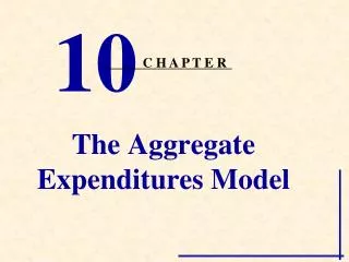
Consumption and Saving Plans Disposable income is either spent on consumption (C) or saved (S), so YD = C + S The relationship between consumption expenditure and disposable income, with other things remaining the same, is called the consumption function. The amount of consumption expenditure that takes place when people have zero income is called autonomous consumption expenditure.
f Saving e Dissaving d c b a Consumption and Saving Plans 500 Consumption function 400 Consumption expenditure (billions of 1995 pounds per year) 300 200 100 0 100 200 300 400 500 Disposable income (billions of 1995 pounds per year)
Consumption and Saving Plans The relationship between saving and disposable income, with other things remaining the same, is called the saving function. Negative saving is called dissaving
Saving function Saving f Dissaving e d c b a Consumption and Saving Plans 100 Saving (billions of 1995 pounds per year) 0 100 200 300 400 500 Disposable income (billions of 1995 pounds per year) -100
Marginal Propensity to Consume The marginal propensity to consume (MPC) is the fraction of a change in disposable income that is consumed. MPC= ΔC ΔYd
f MPC= 0.75 e d c billion b billion a 45o line 500 Consumption function 400 Consumption expenditure (billions of 1992 pounds per year) 300 200 100 0 100 200 300 400 500 Disposable income (billions of 1992 pounds per year)
Marginal Propensity to Save The marginal propensity to save (MPS) is the fraction of a change in disposable income that is saved. MPS= ΔS ΔYd
MPC AND MPS Because consumption expenditure and saving exhaust disposable income, the marginal propensity to consume plus the marginal propensity to save always equals 1. ΔC + ΔS = ΔYd Dividing both sides by DYD ΔC + ΔS = ΔYd ΔYd ΔYd ΔYd MPC + MPS = 1
The Aggregate Expenditure Model Aggregate planned expenditure is planned consumption expenditure plus planned investment plus planned government expenditures plus planned exports minus planned imports. Planned consumption expenditure and planned imports are influenced — and influence — real GDP
The Aggregate Expenditure Model The aggregate expenditure schedule lists aggregate planned expenditure generated at each level of real GDP. Aggregate planned expenditure increases as real GDP increases. However, only consumption expenditure and imports increase with real GDP. Induced expenditure is the sum of the components of aggregate expenditure that vary with real GDP. Autonomous expenditure is the sum of the components of aggregate expenditure that are not influenced by real GDP.
Planned expenditure Aggregate Consumption Government planned Real GDP expenditure Investment purchases Exports Imports expenditure (Y) (C) (I) (G) (X) (M) (AE=C+I+G+X–M) 0 0.75 0.5 0.55 1.2 0.0 3 2 2.25 0.5 0.55 1.2 0.5 4 4 3.75 0.5 0.55 1.2 1.0 5 6 5.25 0.5 0.55 1.2 1.5 6 8 6.75 0.5 0.55 1.2 2.0 7 10 8.25 0.5 0.55 1.2 2.5 8 (trillions of 1992 dollars)
Change in equilibrium expenditure Multiplier = Change in autonomous expenditure £200 billion = = 4 £50 billion The Size of the Multiplier The multiplier is the amount by which a change in autonomous expenditure is multiplied to determine the change in equilibrium expenditure that it generates.
The Multiplier and the Slope of the AE Curve The slope of the AE curve determines the magnitude of the multiplier. The steeper the AE curve, the greater is the increase in induced expenditure that results from a given increase in real GDP. Multiplier =ΔY = 1 ΔA 1- Slope of AE curve If the slope of the AE curve is 0.75: Multiplier = 1 = 1 = 4 1- 0.75 0.25
The Algebra of the Multiplier Symbols: • Aggregate planned expenditure, AE • Real GDP, Y • Consumption expenditure, C • Investment, I • Government expenditures, G • Exports, X • Imports, M • Net taxes, NT • Disposable income, YD • Autonomous consumption expenditure, a • Marginal propensity to consume, b • Marginal propensity to import, m • Marginal tax rate, t • Autonomous expenditure expenditures, A
Aggregate Expenditure Aggregate expenditure is the sum of planned amounts of consumption expenditure, investment, government expenditures, and exports minus the planned amount of imports: AE = C + I + G + X – M We write the consumption function as: C = a + bYd
Autonomous expenditure (A) Slope of the AE curve Equilibrium Expenditure Grouping together terms that involve Y we obtain: AE = [a + I + G + X] + [b(1 – t) – m]Y
Equilibrium Expenditure Equilibrium expenditure occurs when aggregate planned expenditure equals real GDP: AE = Y To calculate equilibrium expenditure and real GDP, we solve the equation for the AE curve and the 45º line for AE and Y: AE = A + [b(1 –t) – m]Y AE = Y
Equilibrium Expenditure ReplaceAE with Yin the AE equation to obtain: Y = A + [b(1 – t) – m]Y or