Sequence Analysis Methods for comparative Genomics
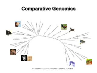
Sequence Analysis Methods for comparative Genomics. Philipp Bucher. Comparative Genomics SIB PhD program Lausanne Feb 12-16 2007. Topics covered. Alignment methods for genomic DNA sequences Comparative gene prediction Comparative motif finding. Genome sequence comparison - Challenges.

Sequence Analysis Methods for comparative Genomics
E N D
Presentation Transcript
Sequence Analysis Methods for comparative Genomics Philipp Bucher Comparative Genomics SIB PhD program Lausanne Feb 12-16 2007
Topics covered Alignment methods for genomic DNA sequences Comparative gene prediction Comparative motif finding
Genome sequence comparison - Challenges Very large sequences – up to several 100 million bp per chromosome Only a small percentage of the genomes may be alignable. Chromosomal rearrangements: • Insertions • Translocations • Duplications Repetitive elements: • simple repeats • lineage specific transposons • ancient transposons • Processed pseudogenes
Nothing in biology makes sense except in the light of evolutionTh. Dobzhansky In fact, many contemporary biologists don’t care about evolution but are more interested in molecular function or drug discovery. To those, comparative genomics is an extremely powerful genome annotation technique. Genome sequence comparison may helpful in: the assembly of a new genomes predicting gene structures the identification of non-coding regulatory elements In the recognition of orthologs to discarding sequence regions not of interest in a particular context for structural and functional inferences from substitution patterns
BLAST heuristics for protein sequence similarity searches 1. Query compilation: For each position of the query sequence, compile a list of 3-letter words which match the query with score threshold T (score depends on substitution matrix). 2. Word search: Search for two non-overlapping word matches on the same diagonal of the path matrix within a distance A. 3. Un-gapped match extension: Extend the un-gapped alignment along the diagonal in both directions unless the score drops more than X below the maximal score yet attained. 4. Gapped alignment extension: For un-gapped alignments (segment pairs) exceeding a threshold score Sg , trigger a regional gapped alignment until the score drops more than Xg below the maximal score yet attained. 5. Statistical evaluation of gapped alignments: Blast uses hard-wired extreme value distribution parameters λ and K for specific scoring systems (substitution matrix + gap penalties)
Examples of word match scores with Blosum62 matrix WWW -> 33 WWW YYY -> 21 YYY GGG -> 18 GGG QQQ -> 15 QQQ SSS -> 13 SSS HSW -> 20 HAW LFY -> 12 IYY EWD -> 15 DWE KFI -> 8 RYV EWC -> -11 FDE # Matrix made by matblas from blosum62.iij # * column uses minimum score # BLOSUM Clustered Scoring Matrix in 1/2 Bit Units # Blocks Database = /data/blocks_5.0/blocks.dat # Cluster Percentage: >= 62 # Entropy = 0.6979, Expected = -0.5209 A R N D C Q E G H I L K M F P S T W Y V B Z X * A 4 -1 -2 -2 0 -1 -1 0 -2 -1 -1 -1 -1 -2 -1 1 0 -3 -2 0 -2 -1 0 -4 R -1 5 0 -2 -3 1 0 -2 0 -3 -2 2 -1 -3 -2 -1 -1 -3 -2 -3 -1 0 -1 -4 N -2 0 6 1 -3 0 0 0 1 -3 -3 0 -2 -3 -2 1 0 -4 -2 -3 3 0 -1 -4 D -2 -2 1 6 -3 0 2 -1 -1 -3 -4 -1 -3 -3 -1 0 -1 -4 -3 -3 4 1 -1 -4 C 0 -3 -3 -3 9 -3 -4 -3 -3 -1 -1 -3 -1 -2 -3 -1 -1 -2 -2 -1 -3 -3 -2 -4 Q -1 1 0 0 -3 5 2 -2 0 -3 -2 1 0 -3 -1 0 -1 -2 -1 -2 0 3 -1 -4 E -1 0 0 2 -4 2 5 -2 0 -3 -3 1 -2 -3 -1 0 -1 -3 -2 -2 1 4 -1 -4 G 0 -2 0 -1 -3 -2 -2 6 -2 -4 -4 -2 -3 -3 -2 0 -2 -2 -3 -3 -1 -2 -1 -4 H -2 0 1 -1 -3 0 0 -2 8 -3 -3 -1 -2 -1 -2 -1 -2 -2 2 -3 0 0 -1 -4 I -1 -3 -3 -3 -1 -3 -3 -4 -3 4 2 -3 1 0 -3 -2 -1 -3 -1 3 -3 -3 -1 -4 L -1 -2 -3 -4 -1 -2 -3 -4 -3 2 4 -2 2 0 -3 -2 -1 -2 -1 1 -4 -3 -1 -4 K -1 2 0 -1 -3 1 1 -2 -1 -3 -2 5 -1 -3 -1 0 -1 -3 -2 -2 0 1 -1 -4 M -1 -1 -2 -3 -1 0 -2 -3 -2 1 2 -1 5 0 -2 -1 -1 -1 -1 1 -3 -1 -1 -4 F -2 -3 -3 -3 -2 -3 -3 -3 -1 0 0 -3 0 6 -4 -2 -2 1 3 -1 -3 -3 -1 -4 P -1 -2 -2 -1 -3 -1 -1 -2 -2 -3 -3 -1 -2 -4 7 -1 -1 -4 -3 -2 -2 -1 -2 -4 S 1 -1 1 0 -1 0 0 0 -1 -2 -2 0 -1 -2 -1 4 1 -3 -2 -2 0 0 0 -4 T 0 -1 0 -1 -1 -1 -1 -2 -2 -1 -1 -1 -1 -2 -1 1 5 -2 -2 0 -1 -1 0 -4 W -3 -3 -4 -4 -2 -2 -3 -2 -2 -3 -2 -3 -1 1 -4 -3 -2 11 2 -3 -4 -3 -2 -4 Y -2 -2 -2 -3 -2 -1 -2 -3 2 -1 -1 -2 -1 3 -3 -2 -2 2 7 -1 -3 -2 -1 -4 V 0 -3 -3 -3 -1 -2 -2 -3 -3 3 1 -2 1 -1 -2 -2 0 -3 -1 4 -3 -2 -1 -4 B -2 -1 3 4 -3 0 1 -1 0 -3 -4 0 -3 -3 -2 0 -1 -4 -3 -3 4 1 -1 -4 Z -1 0 0 1 -3 3 4 -2 0 -3 -3 1 -1 -3 -1 0 -1 -3 -2 -2 1 4 -1 -4 X 0 -1 -1 -1 -2 -1 -1 -1 -1 -1 -1 -1 -1 -1 -2 0 0 -2 -1 -1 -1 -1 -1 -4 * -4 -4 -4 -4 -4 -4 -4 -4 -4 -4 -4 -4 -4 -4 -4 -4 -4 -4 -4 -4 -4 -4 -4 1
Blast: Gap extension. a: Area considered by gap extension algorithm. Computation starts at the center of the highest scoring segment pair obtained after word-hit extension. b: Path of optimal local alignment found. c: Optimal local alingment.
Blastz overview: Searches for multiple gapped local alignments • ordering constraints may apply Same 3-step procedure as blast: • word hit, ungapped extension, gapped extension Word hits: • exact (default 8) or patterned, e.g. 1110100110010101111 (1 indicates relevant positions). • optionally transition-tolerant (A:G, C:T count as matches) • two hits strategy like blastp Species-pair specific base substitution matrix Alignment scores dynamically adjusted for local complexity Between adjacent alignments: search repeated with more sensitive parameters Output: • Coordinates of local alignments and scores • For each alignment, coordinates and scores of HSPs (high-scoring segment pairs)
Comparative gene prediction: Categories of gene prediction programs: • Single-genome ab initio (classical gene prediction problem) • Dual-genome ab initio (comparative gene prediction) • EST-, mRNA, and protein-based methods (same or related species) • Anything goes (e.g. ENSEMBL gene annotation pipeline) Why should comparative gene prediction be more effective: • Consensus of two predictions more reliable than one • Coding regions more conserved than non-coding regions (??) • Coding regions have different substitution and indel patterns (frame conservation) • Splice junctions need to be conserved as well Some limitations: • Genomes need to be reasonably diverse • Gene structures may not be conserved
Gene prediction: statement of the problem • Given a genome sequence: • predict the structure of all transcripts • Predict the structure of the coding part of all transcripts. • Performance criteria: • # of correctly predicted/missed genes • # of correctly predicted/missed exons • # of correctly predicted/missed coding nucleotides • Further complications: • It is not known in advance how many genes a sequence contains • The sequence may start or end in the middle of a gene • Alternative splicing
GENSCAN, and example of an ab initio gene finding algorithm • Principle: GENSCAN finds the optimal “parse” of a sequence • A “parse” is a succession of: • intergenic regions • 5’UTR (untranslated regions) • Exons • Introns • 3’UTRs • Evaluation of alternative parses with the aid of: • Weight matrices or similar models for sites: promoters, translation starts, splice donors and acceptors, translation stops, polyadenylation sites. • Interpolated Markov chains (3-periodic HMMs), and length distributions for exons, introns, 5’ and 3’ UTRs, and intergenic regions.
GENESCAN model (variant HMM) E0+ = exon + plus starting in phase 0 I0+ = exon on + starting in phase 1 All named elements except promoters are scored by Markov chains or interpolated Markov chains. Transitions and promoters are scored by weight matrices or similar descriptors
Gene Prediction: The Intron Phase Problem ATGGGTCCAgttggtgcccttagGTGTTCGAgtgagccacagCACCTGGAAG MetGlyPro..............ValTyrAs...........pThrTrpLys EInit I0+ E0+ I2+ E2+ • Introns can be inserted at three different codon positions: • Introns inserted between codons have phase 0 • Introns inserted after the first codon base have phase 1 • Introns inserted after the second codon position have phase 2 • Exons starting between codons have phase 0 • Exons starting after the first codon base have phase 1 • Exons starting after the second codon base have phase 2 • Important rule: An intron of a given phase must be followed by an exon of the same phase. Otherwise, the protein will not be translated in the correct frame.
Scoring target Scoring method: • F+ 5’UTR simple Markov chain • F+→ Einit+ Kozak consensus weight matrix • Einit First exon interpolated Markov chain • Einit → I1+ Splice donor weigh matrix • I1+Intron phase 1 interpolated Markov chain • I1 + → E1+ Splice acceptor weigh matrix - like
Example of a dual gene prediction program: SLAM Input: • two sequences • Approximate alignments generated with Avid or Mummer Coupled gene prediction and alignment optimization Based on a generalized pair HMM (GPHMM) • gene model analogous to GENSCAN • arbitrary length distributions (two sets of durations instead of one) • exon model based on codon pairs in different alignment configurations (new!) • Splice junctions modeled by VLMMs (non-stationary variable-length Markov models) Models individually trained for different species Other examples of dual gene prediction programs: • SGP2 • TWINSCAN
Evaluation of gene predictions(from Guigo et al. 2006, Genome Biol. 7:S2)
Evaluation at gene level Gene transcript evaluation. Computing sensitivity and specificity at transcript level: (a) complete transcript annotation; (b) incomplete transcript annotation. Transcripts marked with an asterisk are considered 'consistent with the annotation' and will be scored as correct.
Performance Evaluation of gene prediction programs based on experimentally characterized EGASP regions
Computational Approaches to Gene Regulatory elements Commonly addressed problems and corresponding bottlenecks: • Finding a common sequence motif in a set of sequences known to contain a binding site to the same transcription factor or to confer the same regulatory property to an adjacent gene. Bottleneck: appropriate data sets, computer algorithms. New perspective: ChIP-chip data. • Identification of sequence motifs that are over-represented at a particular distance from transcription initiation sites. Bottleneck: large sets of experimentally mapped promoters. Hope comes from mass genome annotation (MGA) data (CAGE, etc.). • Identification of transcription factor binding sites and other sequence elements in DNA regulatory sequences. Bottleneck: accurate and reliable motif descriptions. • Development of promoter prediction algorithms. Current bottleneck: large sets of experimentally mapped promoters. Perspective: MGA data. • Identification and interpretation of conserved non-coding sequence regions between orthologous genes of related organisms. Current bottleneck: concepts and models of gene regulatory regions. Comparative genomics may help solving these problems
Transcription Factor Binding Sites: Features and Facts Degenerate sequence motifs Typical length: 6-20 bp Low information content: 8-12 bits (1 site per 250-4000 bp) Quantitative recognition mechanism: measurable affinity of different sites may vary over three orders of magnitude Regulatory function often depends on cooperative interactions with neighboring sites
Limitations of Motif Discovery Algorithms A recent paper show that computational motif discovery is disappointingly ineffective:
Bad Performance of Motif Discovery algorithms on Eukaryotic Benchmark Data Sets (Results from Tompa et. al. 2005)
Similar results are obtained with prokaryotic benchmark datasets
Comparative Motif Discovery: Problem statement and strategies • Problem 1: Motif discovery • Input: several sets of aligned or unaligned sequences. • Output: a set of over-, under-, or class-associated motifs • Motifs may be represented as consensus sequences or weight matrices • Case study: Xie et al. (2005) mammalian promoters and 3’UTRs • Program example: PhyloGibbs (Siddhartan et al. 2005) • http://www.phylogibbs.unibas.ch/cgi-bin/phylogibbs.pl • Problem 2: Motif search • Input: one set of aligned or unaligned sequences, a library of motif definitions (e.g. TRANSAC matrices) • Output: conserved binding site locations • Program example: ConSite (Sandelin et al. 2004), CisOrtho (Bigelow et al. 2004)
New human promoter motifs discovered by comparative approach Data from Xie et al. 2005, Nature 434, 338-345