Download
1 / 12
130 likes | 318 Vues
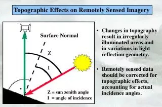
Topographic Effects on Remotely Sensed Imagery. Changes in topography result in irregularly illuminated areas and in variations in light reflection geometry. Remotely sensed data should be corrected for topographic effects, accounting for actual incidence angles. Surface Normal.

E N D
Topographic Effects on Remotely Sensed Imagery • Changes in topography result in irregularly illuminated areas and in variations in light reflection geometry. • Remotely sensed data should be corrected for topographic effects, accounting for actual incidence angles. Surface Normal Z = sun zenith angle I = angle of incidence
Statistical-Empirical Correction for Topographic Effects Illumination: cos(i) = cos(e) cos (z) + sin(e) sin (z) cos (Øs - Øn) i = angle of incidence e = surface slope z = solar zenith angle Øs= solar azimuth angle Øn= surface aspect } at time of satellite overpass Observed radiance: LOBS = b + m cos(i) Corrected radiance: LCOR = LOBS - m cos(i) - b + LOBS, avrg LOBS = observed radiance (actual terrain) LCOR = corrected radiance (normalized, horizontal surface) m, b = regression coefficients
Observed Radiance: LOBS = b + m cos(i) 120 110 100 90 80 70 60 50 40 30 20 10715 ground reference points (natural forest) b = 74.9 m = 54.1 (band 4) cos(i) 0.0 0.1 0.2 0.3 0.4 0.5 0.6 0.7 0.8 0.9 1.0
Corrected Radiance: LCOR = LOBS - b - m cos(i) + LOBS,avrg 120 110 100 90 80 70 60 50 40 30 20 b = 74.9 m = 54.1 (band 4) 10715 ground reference points (natural forest) cos(i) 0.0 0.1 0.2 0.3 0.4 0.5 0.6 0.7 0.8 0.9 1.0
Digital Elevation Model 1200-1250 1250-1300 1300-1350 1350-1400 1400-1450 1450-1500 1500-1550 1550-1600 1600-1650 1650-1700 1700-1750 1750-1800 1800-1850 1850-1900 1900-1950 1950-2000 2000-2050 2050-2100 2100-2150 2150-2200 2200-2250 2250-2300 2300-2350 (m.a.s.l.)
DEM-based aspect (degrees.) DEM-based slope (degrees.)
Color composite original bands 742 Color composite corrected bands 742
Mitch Langford’s classification Unknown clusters
Airphotography-based land use USC corrected composite 453 Cluster 1 Cluster 2 Cluster 3 Cluster 4 Cluster 5 Cluster 6 Cluster 7 BN BP PNB PBD PC PN MS CC CT FQ CN CI YU PR Q PNC MR MC RA PNE
Mitch Langford’s classification USC corrected composite 453 Cluster 1 Cluster 2 Cluster 3 Cluster 4 Cluster 5 Cluster 6 Cluster 7
Conclusions • Satellite imagery of mountainous regions should be corrected for topographic effects before using any further. • The statistical-empirical correction method using DEM-derived information proved to be effective and easy. • The spatial resolution of imagery (30 m) may be insufficient to identify many small plots with different land cover. • Image correction and classification can be further improved by using better ground reference information.