
Introducing Non-Linearities
This document explores the introduction of non-linearities in neural networks to achieve complex decision boundaries that are not merely linear. We begin with a linear decision boundary equation and transition to an elliptical boundary using non-linear transformations. The architecture includes non-linear neurons designed for tasks like Exclusive OR (XOR). The learning process employs MATLAB to implement the Delta Learning Rule with various training vectors. Lastly, we discuss memory models, pattern associations, and how neural networks can learn and recall based on similarities in input patterns.

Introducing Non-Linearities
E N D
Presentation Transcript
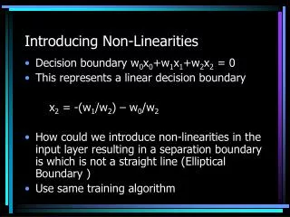
Introducing Non-Linearities • Decision boundary w0x0+w1x1+w2x2 = 0 • This represents a linear decision boundary x2 = -(w1/w2) – w0/w2 • How could we introduce non-linearities in the input layer resulting in a separation boundary is which is not a straight line (Elliptical Boundary ) • Use same training algorithm
Non-Linearities • Introduce non-linearities The following equation represents an ellipse in the two dimensional input vector space: w0 + w1x12 + w2x1 + w3x1x2 + w4x2 + w5x22 = 0
Non-linear Neuron Architecture x0 x1 x12 x2 x22 x1x2 y
Non Linear Neuron - Exclusive OR X = [ 1, -1, -1 +1, +1, +1; %Training Vectors 1 -1, +1 +1, +1, -1; 1, +1, -1 +1, +1, -1; 1, +1, +1 +1, +1, +1]'; t = [ -1, 1, 1, -1]; %Target Values alpha = .01 ; % Learning rate
Reading Assignment • Finish reading chapter 2 ( skip section 2.4.5 ) • Quiz on Tuesday
Assignment #2 Due: Thursday, January 10th • PART 1 of 2 Parts • Program the Delta Learning Rule in MATLAB • Use following parameters ( AND Function ): X = [ 1, -1, -1; %Training Vectors 1 -1, +1; 1, +1, -1; 1, +1, +1 ]'; t = [ -1, 1, 1, 1]; %Target Values alpha = .01 ; % Learning rate Experiment with tolerance and learning rate. Does it find the correct weights every time? Plot final boundary
Example of 2D plotting Script %plotBoundary.m % Roger S. Gaborski, December 19, 2001 % reads in weights and plots 2D boundary % Wn %weights x1 = [-2: .5: 2]; x2= -1*(Wn(2)/Wn(3))*x1 -(Wn(1)/Wn(3)) %Wn indices larger than notes because % matrix starts at index 1 instead of zero plot(x1,x2), axis([-2,2,-2,2]) grid hold on plot(1,1,'*') plot(1, -1, '*') plot(-1, 1, '*') plot(-1, -1, 'o')
Assignment #2 Due: Thursday, January 10th • Part 2 • Implement the Exclusive OR using nonlinearities • Create 3D plot and thresholded 2D shown in previous slides
Assignment #2 Due: Thursday, January 10th • Write up observations • Turn in: hardcopy of MATLAB code • Email MATLAB scripts and directions rsg@cs.rit.edu
Memory • Content Addressable • Distributed, robust, noise tolerant • Fast retrieval • Adaptive
Memory Model Memory Model Two input patterns mapped to this pattern M’ output patterns Learning Stage M input patterns
Memory • If input is noisy, distorted or only partial information available the memory model will respond with the “output” to correct output
Memory Model Memory Model Similar Pattern M’ output patterns
Memory Damage Memory Model Similar Pattern M’ output patterns
Memory Damage 100% % Accuracy 0 % % Damage
Pattern Association • Learning – form associations between patterns • Visual image associated with another visual image ( recognize a person we have only seen in a photograph ) • Visual image associated with a smell ( beach scene coconut smell (suntan oil)) - Music a few notes artist events when ong as popular where you lived, job, chool
Pattern Association • Single Layer Neural Network • Store associations • Retrieve information based on content rather than computer memory address • Information is distributed in the weights Does not have ‘specific’ storage address
Pattern Associations • How are ‘associations’ different that classification neural networks?? • No thresholding into different classes • Output usually a vector • Not always ‘single forward pass’. Sometime an iterative operation is employed
Pattern Association • Each association is an Input : Output vector pair s:t • If s = t, autoassociative memory • If s t, heteroassociative memory Not only learns specific pairs used in training, but able to recall a stimulus that is similar, but NOT identical
Heteroassociative Memory s t • Each association is a pair of vectors ( s(p) , t(p) ) p=1,2,3,…P • Each vector s(p) is an n-tuple • Each vector t(p) is an m-tuple • Weights can be found using either the Hebb Rule or the Extended Delta Rule
Hebb Rule for Pattern Association • Use either binary or bipolar vectors • Training vector pairs s:t • Testing Input Vector x • Procedure: • Initialize all weights to 0, wij = 0, ( i = 1,…,n; j = 1,…,m) • For each training pair: • Set activations for input neurons to current training input ( i = 1, …, n ): xi = si • Set activation for output neurons to current target output ( j = 1,…,m): yj = tj • Update weights: wij(new) = wij(old) + xiyj
Hebb Rule using Outer Products • For individual input / output pair: s = ( s1, …, si , … sn ) 1xn vector t = ( t1, …, tj ,… tm ) 1xm vector S = s’S is nx1 after transpose T = t T is still 1xm, no transpose ST = s1 . . sn s1t1 … s1tj… s1tm . . . snt1 … sntj… sntm t1, … , tm = 1xm nx1
Hebb Rule using Outer Products • For a set of Associations s(p):t(p) W = s’(p) t(p) p p=1 Just sum weight matrices for each pair
Heteroassociative Memory w11 Y1 Yj Ym X1 Xi Xn Output vector y is the pattern associated with input vector x w1j w1m
Hebb Learning for Heteroassociative Memory • Step 1: Initialize weights • Step 2: For each input vector • Set activations for input layer equal to the current input vector • Compute net input to output neurons y_inj = xiwij • Determine activation of output units 1 if y_inj >0 yj = 0 if y_inj = 0 -1 if y_inj < 0
Example of Hebb Outer Product Rule for Heteroassociative Memory - 1 Input row vectors s = ( s1, s2, s3, s4 ) Output vectors t = ( t1, t2 ) s1 = ( 1, 0, 0, 0 ) t1 = ( 1, 0 ) s2 = ( 1, 1, 0, 0 ) t2 = ( 1, 0 ) s3 = ( 0, 0, 0, 1 ) t3 = ( 0, 1 ) s4 = ( 0, 0, 1, 1 ) t4 = ( 0, 1 ) 1 0 0 0 1 0 0 0 0 0 0 0 1 1 0 0 • 0 • 1 0 • 0 0 • 0 0 1 0 1 0 = =
Example of Hebb Outer Product Rule for Heteroassociative Memory - 2 0 0 0 0 0 1 0 1 0 0 0 1 0 0 0 0 0 0 0 1 0 0 1 1 0 1 0 1 = = The weight matrix to store all four patterns is simply the Sum of the four individual patterns 2 0 1 0 0 1 0 2 W=
Example of Hebb Outer Product Rule for Heteroassociative Memory – 3 TESTING Test on training date: W = x= ( 1, 0,0,0 ) 2 0 1 0 0 1 0 2 2 0 1 0 0 1 0 2 = ( 1, 0,0,0 ) = (2,0 ) xW = ( y_in1, y_in2 ) f(2) = 1, f(0) = 0, y = ( 1,0 )
Example of Hebb Outer Product Rule for Heteroassociative Memory – 4 TESTING f ( 1, 0, 0, 0 )W = ( 2,0 ) (1,0 ) where f is the activation function Test on new data similar to training date: ( 0,1,0,0 ) W = ( 1,0 ) ( 1,0 ) Is this a reasonable response?? Original Data: s1 = ( 1, 0, 0, 0 ) t1 = ( 1, 0 ) s2 = ( 1, 1, 0, 0 ) t2 = ( 1, 0 ) s3 = ( 0, 0, 0, 1 ) t3 = ( 0, 1 ) s4 = ( 0, 0, 1, 1 ) t4 = ( 0, 1 )
Example of Hebb Outer Product Rule for Heteroassociative Memory – 5 TESTING Hamming distance is a measure of how different two digital Words are. Simply count the number of places where the words differ Input codeword: (0,1,0,0) s1 = ( 1, 0, 0, 0 ) hamming distance = 2 s2 = ( 1, 1, 0, 0 ) hamming distance = 1 s3 = ( 0, 0, 0, 1 ) hamming distance = 2 s4 = ( 0, 0, 1, 1 ) hamming distance = 3 The second codeword is closest to the input word, and its Recall word is ( 1,0 )
Example of Hebb Outer Product Rule for Heteroassociative Memory – 6 TESTING Consider: ( 0, 1,1, 0) This codeword differs in two positions s1 = ( 1, 0, 0, 0 ) hamming distance = 3 s2 = ( 1, 1, 0, 0 ) hamming distance = 2 s3 = ( 0, 0, 0, 1 ) hamming distance = 3 s4 = ( 0, 0, 1, 1 ) hamming distance = 2 (0, 1, 1, 0)W = (1,1) (1,1) Not a valid stored word- FAILS
Bipolar vs Binary Bipolar data gives you the ability to represent unknown (noisy data) with a 0, and good data with +1 or –1
How well does it work?? • If input vectors are orthogonal, the Hebb rule will produce the correct weights. • Testing on training vectors will result in the expected answer ( scaled by the square of the norm of the input vector, where the norm is the inner product with itself ) • Details: • Recall, two vectors s(k) and s(p), kp, that are orthogonal have a dot product = 0 s(k) s’(p) = 0 n si(k) si(p) = 0 i=1
How well does it work – 2 ?? Calculate Weight matrix:W = s’(p) t(p) The net response to an input is: y = xW If the input vector is he kth training vector, x = s(k) s(k)W = s(k)s’(p)t(p)= s(k)s’(k)t(k) + s(k)s’(p)t(p) Where: s(k)s’(k)t(k) is target t(k) scaled by square of norm of s(k) And:s(k)s’(p)t(p) if s(k) is orthogonal to s(p) this term is 0 pk pk
Delta Rule for Pattern Association • Recall Hebb learning is a ‘one pass’ learning process. • Delta Rule is an iterative learning process • Can be used for input patterns that are linearly independent, but not orthogonal • Avoids difficulty of cross talk which is encountered in Hebb Rule • Delta Rule produces least square solution when input patterns are not linearly independent
Extended Delta Rule • The original Delta Rule used the identity function for the activation function of the output neuron resulting in: wij = ( tj – yj ) xi • The Extended Delta Rule uses a differentiable activation function resulting in: wIJ = ( tJ – yJ ) xI f ’( y_inJ ) This is the update for the weight between neuron I and J