Action Research Data Manipulation and Crosstabs
570 likes | 716 Vues
Action Research Data Manipulation and Crosstabs. INFO 515 Glenn Booker. Parametric vs. Nonparametric. Statistical tests fall into two broad categories – parametric & nonparametric Parametric methods Require data at higher levels of measurement - interval and/or ratio scales

Action Research Data Manipulation and Crosstabs
E N D
Presentation Transcript
Action ResearchData Manipulation and Crosstabs INFO 515 Glenn Booker Lecture #8
Parametric vs. Nonparametric • Statistical tests fall into two broad categories – parametric & nonparametric • Parametric methods • Require data at higher levels of measurement - interval and/or ratio scales • Are more mathematically powerful than nonparametric statistics • But often require more assumptions about the data, such as having a normal distribution, or equal variances Lecture #8
Parametric vs. Nonparametric • Nonparametric methods • Use nominal or ordinal scale data • Still allows us to test for a relationship, and its strength and direction (direction only if ordinal) • Often has easier prerequisites for being tested (e.g. no distribution limits) • Ratio or interval scale data may be recoded to become nominal or ordinal data, and hence be used with nonparametric tests Lecture #8
Significance and Association • … are useful for inferring population values from samples (inferential statistics) • Significance establishes whether chance can be ruled out as the most likely explanation of differences • Association shows the nature, strength, and/or direction of the relationship between two (or among three or more) variables • Need to show significance before association is meaningful Lecture #8
Common Tests of Significance • We’ve been introduced to three common tests of significance: • z test (large samples of ratio or interval data) • t test (small samples of ratio or interval data) • F test (ANOVA) • Shortly we’ll explore a fourth one • Pearson’s chi-square 2 (used for nominal or ordinal scale data) { is the Greek letter chi, pronounced ‘kye’, rhymes with ‘rye’} Lecture #8
Common Measures of Association • Association measures often range in valuefrom -1 to +1 (but not always!) • Absence of association between variables generally means a result of 0 • Examples • Pearson’s r (for interval or ratio scale data) • Yule’s Q (ordinal data in a 2x2 table) • Gamma (ordinal – more than 2x2 table) {A “2x2” table has 2 rows and 2 columns of data.} Lecture #8
Common Measures of Association • Notice these are all for nominal scale data • Phi (, ‘fee’) (nominal data in a 2x2 table) • Contingency Coefficient (nominal – table larger than 2x2) • Cramer’s V (nominal - larger than 2x2) • Lambda (l) - nominal data • Eta () – nominal data Lecture #8
Significance and Association • Tests of significance and measures of association are often used together • But you can have statistical significance without having association Lecture #8
Significance and Association Examples • Ratio data: You might use F to determine if there is a significant relationship, then use ‘r’ from a regression to measure its strength • Ordinal data: You might run a chi-square to determine statistical significance in the frequencies of two variables, and then run a Yule’s Q to show the relationship between the variables Lecture #8
Crosstabs • Brief digression to introduce crosstabs before discussing non-parametric methods • Crosstabs are a table, often used to display data, sorted by two nominal or ordinal variables at once, to study the relationship between variables that have a small number of possible answers each • Generally contains basic descriptive statistics, such as frequency counts and percentages Lecture #8
Crosstabs • Used to check the distribution of data, and as a foundation for more complex tests • Look for gaps or sparse data (little or no contribution to the data set) • Rule of thumb - put independent variable in the columns and dependent variable in the rows Lecture #8
Percentages • Can show both column and row percentages in crosstabs, rather than just frequency counts (or show both counts and percentages) • Make sure percentages add to 100%! • Raw frequency counts of variables don’t always provide an accurate picture • Unequal numbers of subjects in groups (N) might make the numbers appear skewed Lecture #8
Crosstabs Example • Open data set “GSS91 political.sav” • Use Analyze / Descriptive Statistics / Crosstabs... • Set the Row(s) as “region”, and the Column(s) as “relig” • Note the default scope of an SPSS crosstab is to show frequency Counts, with row and column totals Lecture #8
Crosstabs Example Lecture #8
Crosstabs Example • Repeat the same example with percentages selected under the “Cells…” button to get detailed data in each cell • Percent within that region (Row) • Percent within that religious preference (Column) • Percent of total data set (divide by Total N) • Gets a bit messy to show this much! Lecture #8
Crosstabs Example Lecture #8
Recoding • An interval or ratio scaled variable, like age or salary, may have too many distinct values to use in a crosstab • Recoding lets you combine values into a single new variable -- also called collapsing the codes • Also helpful for creating histogram variables (e.g. ranges of age or income) Lecture #8
Recoding Example • Use Transform / Recode / Into Different Variables… • Move “age” from the dropdown list for the Numeric Variable • Define the new Output Variable to have Name “agegroup” and Label “Age Group” • Click “Change” button to use “agegroup” • Click on “Old and New Values” button Lecture #8
Recoding Example • For the Old Value, enter Range of 18 to 30 • Assign this to a New Value of 1 • Click on “Add” • Repeat to define ages 31-50 as agegroup New Value 2, 51-75 as 3, and 76-200 as 4 • Click “Continue” and now a new variable exists as defined Lecture #8
RecodingExample Lecture #8
Recoding Example • Now generate a crosstab with “agegroup” as columns, and “region” as the rows Lecture #8
Second Recoding Example • Prof. Yonker had a previous INFO515 class surveyed for their height (in inches) and desired salaries ($/yr) • Rather than analyze ratio data with few frequencies larger than one, she recoded: • Heights into: Dwarves for people below average height, and Giants for those above • Desired salaries were recoded into Cheap and Expensive, again below and above average Lecture #8
Second Recoding Example • The resulting crosstab was like this: Lecture #8
Pearson Chi Square Test • The Chi Square test measures how much observed (actual) frequencies (fo) differ from “expected” frequencies (fe) • Is a nonparametric test, a.k.a. the Goodness of Fit statistic • Does not require assumptions about the shape of the population distribution • Does not require variables be measured on an interval or ratio scale Lecture #8
Chi Square Concept • Chi Square test is like the ANOVA test • ANOVA proved whether there was a difference among several means – proved that the means are different from each other in some way • Chi square is trying to prove whether the frequency distribution is different from a random one – is there a significant difference among frequencies? • Allows us to test for a relationship (but not the strength or direction if there is one) Lecture #8
Chi Square Null Hypothesis • Null hypothesis is that the frequencies in cells are independent of each other (there is no relationship among them) • Each case is independent of every other case; that is, the value of the variable for one individual does not influence the value for another individual • Chi Square works better for small sample sizes (< hundreds of samples) • WARNING: Almost any really large table will have a significant chi square Lecture #8
Assumptions for Chi Square • A random sample is the “expected” basis for comparison • Each case can fall into only one cell • No zero values are allowed for the observed frequency, fo • And no expected frequencies, fe, less than one • At least 80% of expected frequencies, fe, should be greater than or equal to five (≥5) Lecture #8
Expected Frequency • The expected frequency for a cell is based on the fraction of things which would fall into it randomly, given the same general row and column count proportions as the actual data set • fe = (row total) * (column total) / N • So if 90 people live in New England, and 335 are in Age Group 1 from a total sample of 1500, then we would expect fe = 90*335/1500 = 20.1 people in that cell See slide 21 Lecture #8
Expected Frequency • So the general formula for the expected frequency of a given cell is: fe = (actual row total)* (actual column total)/N • Notice that this is NOT using the average expected frequency for every cell fe = N / [(# of rows)*(# of columns)] Lecture #8
Calculating Chi Square • The Chi square value for each cell is the observed frequency minus the expected one, squared, divided by the expected frequencyChi square per cell = (fo-fe)2/fe • Sum this for all cells in the crosstab • For the cell on slide 28, the actual frequency was 25, so Chi square for that cell is = (25-20.1)2/20.1 = 1.195 Note: Chi square is always positive Lecture #8
Calculating Chi Square • Page 36/37 of the Action Research handout has an example of chi square calculation, where fo is the observed (actual) frequency fe is the expected frequency • E.g. fe for the first cell is 20*30/60 = 10.0 • Chi square for each cell is (fo-fe)2/fe • Sum chi square for all cells in the table No comments about fe fi fo fum! Is that clear?!?! Lecture #8
Interpreting Chi Square • When the total Chi square is larger than the critical value, reject the null hypothesis • See Action Research handout page 42/43 for critical Chi square (2) values • Look up critical value using the ‘df’ value, which is based on the number of rows and columns in the crosstab: df = (#rows - 1)(#columns - 1) • For the example on slide 21, df = (9-1)(4-1) = 8*3 = 24 Lecture #8
Interpreting Chi Square • Or you can be lazy and use the old standby: • if the significance is less than 0.050, reject the null hypothesis if the significance is less than 0.050, reject the null hypothesisif the significance is less than 0.050, reject the null hypothesisif the significance is less than 0.050, reject the null hypothesis Lecture #8
Chi Square Example • Open data set “GSS91 political.sav” • Use Analyze / Descriptive Statistics / Crosstabs... • Set the Row(s) as “region”, and the Column(s) as “agegroup” • Click on “Statistics…” and select the “Chi-square” test Notice we’re still using the Crosstab command! Lecture #8
Chi Square Example Lecture #8
Chi Square Example • Note that we correctly predicted the ‘df’ value of 24 • SPSS is ready to warn you if too many cells expected a count below five, or had expected counts below one • The significance is below 0.050, indicating we reject the null hypothesis • The total Chi square for all cells is 43.260 Lecture #8
Chi Square Example • The critical Chi square value can be looked up on page 42/43 of Yonker • For df = 24, and significance level 0.050, we get a critical Chi square of 36.415 • Since the actual Chi square (43.260) is greater than the critical value (36.415), reject the null hypothesis • Chi square often shows significance falsely for large sample sizes (hence the earlier warning) Lecture #8
Chi Square Example • What are the other tests? They don’t apply here... • The Likelihood Ratio test is specifically for log-linear models • The Linear-by-Linear Association test is a function of Pearson’s ‘r’, so it only applies to interval or ratio scale variables • Notice that SPSS doesn’t realize those tests don’t apply, and blindly presents results for them… Lecture #8
One-variable Chi square Test • To check only one variable’s distribution, there is another way to run Chi square • Null hypothesis is that the variable is evenly distributed across all of its categories • Hence all expected frequencies are equal for each category, unless you specify otherwise • Expected range can also be specified Lecture #8
Other Chi square Example • Use Analyze / Nonparametric Tests / Chi-square… • NOT using the Crosstab command here • Add “region” to the Test Variable List • Now df is the number of categories in the variable, minus one • df = (# categories) - 1 • Significance is interpreted the same Lecture #8
Other Chi square Example Lecture #8
Other Chi square Example • So in this case, the “region” variable has nine categories, for a df of 9-1 = 8 • Critical Chi square for df = 8 is 15.507, so the actual value of 290 shows these data are not evenly distributed across regions • Significance below 0.050 still, in keeping with our fine long established tradition, rejects the null hypothesis Lecture #8
Whodunit? • The chi-square value by itself doesn’t tell us which of the cells are major contributors to the statistical significance • We compute the standardized residual to address that issue • This hints at which cells contribute a lot to the total chi square Lecture #8
Residuals • The Residual is the Observed value minus the Estimated value for some data point • Residual = fo - fe • If this variable is evenly distributed, the Residuals should have a normal distribution • Plots of residuals are sometimes used to check data normalcy (i.e. how normal is this data’s distribution?) Lecture #8
Standardized Residual • The Standardized Residual is the Residual divided by the standard deviation of the residuals • When the absolute value of the Standardized Residual for a cell is greater than 2, you may conclude that it is a major contributor to the overall chi-square value • Analogous to the original t test, looking for |t| > 2 Lecture #8
Standardized Residual • Extreme values of Standardized Residual (e.g. minimum, maximum) can also help identify extreme data points • The meaning of residual is the same for regression analysis, BTW, where residuals are an optional output Lecture #8
Standardized Residual Example • In the crosstab region-agegroup example • Click “Cells…” and select Standardized Residuals • In this case, the worst cell is the combination W. Nor. Central region - Age Group 4, which produced a standardized residual of 2.1 Lecture #8
Standardized Residual Example Lecture #8
Crosstab Statistics for 2x2 Table • 2x2 tables appear so often that many tests have been developed specifically for them • Equality of proportions • McNemar Chi-square • Yates Correction • Fisher Exact Test Lecture #8
Crosstab Statistics for 2x2 Table • Equality of proportions tests prove whether the proportion of one variable is the same as for two different values of another variable • e.g. Do homeowners vote as often as renters? • McNemar Chi-square tests for frequencies in a 2x2 table where samples are dependent (such as pre-test and post-test results) Lecture #8