Download
1 / 159
1.6k likes | 1.7k Vues
Explore key notions of digital topology and their applications in grayscale image processing, from preserving topology to transforming grayscale images. Learn about milestone contributions and topological properties of grayscale images. Dive deep into applications such as filtering and segmentation.

E N D
Digital topology andcross-section topology for grayscale image processing M. Couprie A2SI lab., ESIEE Marne-la-Vallée, France www.esiee.fr/a2si
« A topologist is interested in those properties of a thing that, while they are in a sense geometrical, are the most permanent- the ones that will survive distortion and stretching. » Stephen Barr,"Experiments in Topology",1964 What is topology ?
Aims of this talk • Present the main notions of digital topology • Show their usefulness in image processing applications • Study some topological properties of digital grayscale images (ie. functions from Zn to Z) • Topology-preserving image transforms • Topology-altering image transforms • Applications to image processing (filtering, segmentation…)
Some milestones • J.C. Maxwell (1870): ‘On hills and dales ’ • A. Rosenfeld (1970’s): digital topology • A. Rosenfeld (1980’s): fuzzy digital topology • S. Beucher (1990): definition of homotopy between grayscale images • G. Bertrand (1995): cross-section topology
Contributors • Gilles Bertrand • Michel Couprie • Laurent Perroton • Zouina Aktouf (Ph.D student) • Francisco Nivando Bezerra (Ph.D student) • Xavier Daragon (Ph.D student) • Petr Dokládal (Ph.D student) • Jean-Christophe Everat (Ph.D student)
Outline of the talk Part 1 • Digital topology for binary images • Applications to graylevel image processing • Cross-section topology for grayscale images • Topology-altering transforms, applications Part 2
Digital topology for binary images • 8-adjacency, 4-adjacency in black: X (object) in white: X (background). • path, connected components
Digital topology for binary images • 8-adjacency, 4-adjacencyin black: X (object) in white: X (background). • path, connected components
Digital topology for binary images • 8-adjacency, 4-adjacency in black: X (object)in white: X (background). • path, connected components
Digital topology for binary images • 8-adjacency, 4-adjacency in black: X (object)in white: X (background). • path, connected components
2 2 3 1 More examples Black:4, white:8 Black:8, white:4
Jordan property • Any simple closed curve divides the plane into 2 connected components.
4-curve 8-curve Jordan property (cont.) • A subset X of Z2 is a simple closed curve if each point x of X has exactly two neighbors in X
Jordan property (cont.) • A subset X of Z2 is a simple closed curve if each point x of X has exactly two neighbors in X Not a 4-curve
Jordan property (cont.) • A subset X of Z2 is a simple closed curve if each point x of X has exactly two neighbors in X Not an 8-curve
Jordan property (cont.) • The Jordan property does no hold if X and its complement have the same adjacency 8-adjacency 4-adjacency
Topology preservation - notion of simple point • A topology-preserving transform must preserve the number of connected components of both X and X. • Definition (2D): A point p is simple (for X) if its modification (addition to X, withdrawal from X) does not change the number of connected components of X and X.
Simple point: examples Set X (black points)
Simple point: examples Simple point of X
Simple point: examples Simple point of X
Simple point: counter-examples Non-simple point (background component creation if deleted)
Simple point: counter-examples Non-simple point (component splitting if deleted)
Simple point: parallel deletion Deleting simple points in parallel may change the topology
Connectivity numbers • T(p)=number of Connected Components of (X - {p}) N(p) where N(p)=8-neighborhood of p • T(p)=number of Connected Components of (X - {p}) N(p)A • Characterization of simple points (local): p is simple iff T(p) = 1 and T(p) = 1 A U U T=2,T=2 T=1,T=1 T=1,T=0 T=0,T=1 Isolated point Interior point
Skeletons • We say that Y is a skeleton of X if Y may be obtained from X by sequential deletion of simple points • If Y is a skeleton of X and if Y contains no simple point, then we say that Y is an ultimate skeleton of X • If Y is a skeleton of X and if Y contains only non-simple points and ‘end points’, then we say that Y is a curve skeleton of X
End points • We say that p is an end point for X if (X - {p}) N(p) contains exactly one point U End point End point (8) Non-end point Non-end point
Skeletons (examples) End points Ultimate skeleton Curve skeleton Original image
Homotopy • We say that X and Y are homotopic (i.e. they have the same topology) if Y may be obtained from X by sequential addition or deletion of simple points
Basic thinning algorithms Ultimate thinning(X) Repeat until stability:Select a simple point p of XRemove p from X Curve thinning(X) Repeat until stability:Select a simple, non-end point p of XRemove p from X
Simple pointsdetectedduring the 1stiteration Candidatesfor the 2nditeration Breadth-first thinning
Breadth-first thinning Breadth-first ultimate thinning(X) T := X ; T’ := Repeat until stability While p T do T := T \ {p} If p is a simple point for X then X := X \ {p} For all q neighbour of p, q X, do T’ := T’ {q}T := T’ ; T’ :=
Directional thinning • (only in 2D) North South East West
Parallel directional algorithm • In 2D, simple and non-end points of the same type (N,S,E,W) can be removed in parallel Directional Curve thinning(X) Repeat until stability: For dir =N,S,E,W Let Y be the set of all simple, non-end points of X of type dir X = X \ Y
Up Does not work in 3D • In 3D, there are 6 principal directions: N,S,E,W,Up,Down
Thinning guided by a distance map • Let X be a subset of Z2, the distance mapDMX is defined by, for all point p:DMX(p) = min{dist(p,q), q not in X}where dist is a distance (e.g. city block, chessboard, Euclidean)
Discrete distances • City block distance (d4) d4(p,q) = length of a shortest 4-path between p and q • Chessboard distance (d8) d8(p,q) = length of a shortest 8-path between p and q
1 1 1 1 1 1 1 1 1 1 1 1 1 2 2 2 2 2 2 1 1 1 2 2 2 2 1 1 1 2 3 3 3 3 2 1 3 3 1 2 2 2 2 1 1 2 3 4 4 3 2 1 3 3 3 3 1 2 2 1 1 2 3 4 4 3 2 1 3 3 1 2 4 4 2 1 1 2 3 3 3 3 2 1 3 3 3 3 1 2 2 1 1 2 3 2 2 3 2 1 1 2 2 2 2 2 2 1 1 2 2 1 1 2 2 1 1 2 1 1 1 1 2 1 1 2 1 1 2 1 1 2 1 1 2 1 1 2 2 1 1 2 2 1 1 1 1 1 1 1 1 1 1 1 1 1 1 1 1 1 1 1 1 1 Discrete distance maps d4 d8
d8 de d4 Discrete and Euclidean distance maps
Thinning guided by a distance map: algorithm Ultimate guided thinning(X) Compute the distance map DMX Repeat until stability:Select a simple point p of X such that DMX(p) is minimalRemove p from X Curve guided thinning(X) Id., replace « simple » by « simple non end »
d8 de d4 Thinning guided by a distance map: results
The 3D case A topology-preserving transform must preserve: • number of connected components of X • number of connected components of X • number of « holes » (or « tunnels »)
3D-skeletons Surface skeleton Ultimate skeleton Curve skeleton Original object
T=1,T=1 T=1,T=2 T=3,T=1 Topological classification of points (G. Bertrand) (2D isthmus) (1D isthmus) (simple point)
3D hole closing • G. Bertrand • Z. Aktouf (Ph. D) • L. Perroton