Download
1 / 1
10 likes | 127 Vues
“IDEAL” EDGES VS. MULTIPLE, CONVERGING EDGES WITH COMPLEX GEOMETRY

E N D
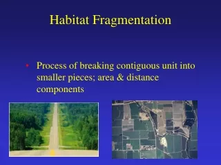
“IDEAL” EDGES VS. MULTIPLE, CONVERGING EDGES WITH COMPLEX GEOMETRY Most studies of edge effects occur at edges that are as “ideal” as possible (a). This means that they are straight, as far as possible away from bends and curves, and usually have only two habitat types on either side of the edge. Even when less-than-ideal edges are studied (as they often are), distance to the closest edge is usually the metric used to assess the magnitude and strength of the edge effects. This measure of edge impact implicitly assumes that edge geometry is simple and only one adjoining habitat type is having an influence. This assumption has rarely been tested either mathematically or empirically. 500m 500m In real landscapes, edges have complex geometry and the convergence of multiple habitat types is common. We show sections of two simplified landscapes that we are using for this project: Ft. Hood in Texas (b) and Ft. Benning in Georgia (c). These landscapes are typical. A recent paper (Li et al. 2007) showed that 60% of their study landscape was within 120m of multiple, converging edges. MALCOLM’S MODEL FOR COMPLEX EDGE GEOMETRY In 1994, Malcolm proposed using line integrals to estimate edge effects. His mathematical model was developed using the biology of edge effects and included three parameters that are the most relevant for any edge study: the density in the core of the habitat, the distance of edge influence (Dmax), and the “point” edge effect, which can be used to calculate edge density. Fernandez et al. (2002) extended the model to allow for multiple edge types. GENERAL APPROACH 1) Decide on your different management options. Develop a series of “alternative scenarios” maps that reflect each option. 2) Using the EAM toolkit, extrapolate known or predicted habitat and edge responses over the alternative maps to predict landscape-wide densities for each species of interest. 3) Use results to help guide management decisions. Malcolm’s model Malcolm only developed and reported the solution for his model along ideal edges in his 1994 paper (a). He then suggested that the model could be applied over any patch shape by breaking the edge into segments and adjusting the limits of integration accordingly. We are not aware of anyone actually applying this model (other than in the original paper). Below we show the solutions to Malcolm’s model along (a) an “ideal” edge (equation 6 from his original paper) and our solution (b) for an “ideal” corner (90o and extending past Dmax in both directions). (b) Solution at an “ideal” corner (90o) (a) Solution at an “ideal” edge y Density = k + L(y) To apply Malcolm’s model in a perfect corner, it is necessary to break the corner into five regions depending on their distance from both edges. The region closest to the origin required a new solution, the others used the equation at left. Dmax is max distance of edge influence, D is distance to edge, e0 is “point edge effect” and k is the density past Dmax, Density = k Dmax Dmax = k + L(x) + L(y) * Density = k + L(x) Dmax Density = k + C(x,y) Where D < Dmax , else k x Dmax This solution was presented in Malcolm (1994) This and all other solutions were left to the reader Modeling the impacts of habitat fragmentation in complex landscapes Leslie Ries1, Emma Goldberg1 & Thomas D. Sisk2 1Department of Biology, University of Maryland, College Park, MD 20742 2Center for Environmental Sciences and Education, Northern Arizona University, Flagstaff, AZ 86011 COULD MALCOLM’S MODEL EVER BE USED ON REAL LANDSCAPES? It is clearly intractable to manually develop solutions to the model for each unique shape on a landscape. To make the use of this model practical, we developed R-scripts that allow the model to be applied to patches of any shape. Results for the golden-cheeked warbler (GCWA) at Ft. Hood in Texas are shown below. OVERVIEW Habitat fragmentation and local land-use decisions are two of the major factors driving habitat quality for threatened and endangered species. However, much of the theory and empirical evidence for how landscape structure impacts habitat quality focuses on highly simplified landscapes. These landscape configurations have practical value in trying to tease apart ecological dynamics within complex systems, but fail when trying to apply the principles in real landscapes. This phenomenon is exemplified by the edge literature, which tends to focus on “ideal” edge geometry. Most focal edges are straight and contain only two adjacent habitat types. Distance to the closest edge is usually the key metric applied. In real landscapes, patches have convoluted, complex shapes where many different habitat types converge, and the distance to the nearest edge may not be the best measure of edge influence. A model published almost 15 years ago (Malcolm 1994) offers a solution, but has never been used because of the difficulty of applying the math to real landscapes. We developed a series of R-scripts to apply this model to any patch shape. We show that including more complex geometry results in subtle, but improved, differences in predictions over traditional models. We discuss the utility of this model in multiple systems and our plans to incorporate a discrete approximation into our Effective Area Model, which is a user-friendly tool that is implemented within ArcGIS. DOES CONSIDERING COMPLEX GEOMETRY IMPROVE SPATIAL PREDICTIONS? For years, researchers have used distance to closest edge as the primary measure for edge effects, ignoring issues of complex geometry and multiple, converging habitat types. Indeed, our spatial model, the Effective Area Model, currently uses distance to closest edge because, at this time, there is simply too little data to justify including more complicated measures. This test represents the first field test of Malcolm’s model in a landscape with complex geometry. To test Malcolm’s model, we selected several survey locations with complex geometry in GCWA habitat on Ft. Hood. However, each location contained only a single edge type within 300 m of the survey point (reflecting the Dmax estimated by the model). We then compared observed GCWA detections to three models: those predicted by Malcolm’s model, those predicted by the distance to nearest edge, and a null model where edge responses are ignored. Golden-cheek warblers in oak-juniper forest APPLYING MALCOLM’S MODEL RESULTED IN SOME IMPROVEMENT FOR GCWAs Incorporating edge responses are critical to understanding GCWA distributions These birds are endemic to central Texas and are federally listed as endangered. The largest population is on Ft. Hood. These birds are highly habitat specific and, using data from Ft. Hood’s extensive network of point surveys, we found that they avoid most other habitat types. We used surveys near the straightest edges to parameterize Malcolm’s equation for ideal edges. The results suggest that natural variation in ecological systems tend to largely trump the fine differences between predictions between the nearest edge and Malcolm’s model. However, there was some improvement. The graph below shows that as edges go from being more concave to more convex, bird detections tend to increase as predicted (with a notable outlier). GCWAs near scrub edges c) habitat configuration in a portion of Ft. Benning b) habitat configuration in a portion of Ft. Hood a) an “ideal” edge Mean number of detections Parameter summary: Dmax = 300m k = 1.1 e0 = -0.002006 This figures shows the predictions of the null (dotted line) and nearest edge (solid line) models, which are easily displayed relative to edge distance. The predictions of Malcolm’s model are shown separately for each survey point (yellow circles). The first pattern to note is that the predictions are not substantially different from the nearest edge model. The observed detection rate (yellow x’s) are clearly much better predicted by a model that includes edge responses (compared to the null model). But does Malcolm’s model improve predictions even more? Distance to closest edge (m) convex concave We then used an optimization program to parameterize the same model, only using the actual edge geometry (which was not perfectly straight or “ideal”). The parameter values changed only slightly (Dmax = 314m, k = 1.1, e0 = -0.001983). We also measured responses along woodland, meadow and large road edges. All showed significant responses in at least some years. • CONCLUSIONS AND FUTURE DIRECTIONS • In addition to the results we present above, we also applied a similar test of Malcolm’s model to black-capped vireos on Ft. Hood and grassland birds in Iowa prairies. We found similar patterns between all three. • Including complex geometry modified predictions only slightly compared to distance to nearest edge measures. • Observed values were often closer to Malcolm’s predictions than nearest edge predictions, suggesting that predictions are somewhat improved by this more complex model. • In many ways these results are encouraging – they suggest that traditional approaches to measuring edge effects are sufficient to capture the dominant shifts in habitat quality as landscapes are modified. They also confirm that incorporating edge effects can substantially improve predictions over null models where edge effects are ignored. • There are still several aspects of complex geometry that need to be considered. When edge effects are very strong, the difference between the nearest edge and Malcolm model increases. For some species, therefore, the impacts of complex geometry may be less trivial. We also have yet to extrapolate these results over an entire landscape, so it is unclear how these differences will accumulate over space. Finally, we have continued to ignore the issue of multiple, converging habitat types. This topic has received no empirical treatment despite decades of edge research and hundreds of published studies. We hope to pursue this topic in the future to determine its impact. • Finally, it is intractable to include Malcolm’s exact model in the EAM, but we are working on developing the model into a discrete version that can more easily be incorporated into a grid-based Arc analytical framework. Based on our current results, we believe that even an approximation would provide value additional information for interested researchers and be sufficient to capture the dynamics of the original model. LITERATURE CITED Li, Q, J Chen, B Song, JJ LaCroix, MK Bresee, and JA Radmacher. 2007. Areas influenced by multiple edges and their implications in fragmented landscapes. For Ecol and Mgt 242:99-107 Fernandez C, FJ Acosta, G Abella, F. Lopez, and M. Diaz. 2002. Complex edge effect fields as additive processes in patches of ecological systems. Ecol. Model. 149:273-83. Fletcher RJ, L Ries, J Battin and AD Chalfoun 2007. The role of habitat area and edge in fragmented landscapes: definitively distinct or inevitably intertwined? Can. J. Zool. 85:1017-1030. Haddad, NM and KA Baum 1999. An experimental test of corridor effects on butterfly densities. Ecol. Appl. 9:623-633. Malcolm, JR. 1994. Edge effects in central Amazonian forest fragments. Ecology 75:2438-45. Ries, L, RJ Fletcher, J Battin, and TD Sisk 2004. Ecological responses to habitat edges: Mechanisms, models and variability explained. Ann. Rev. Ecol. Evol. Syst. 35:491-522. WHY FOCUS ON HABITAT AND EDGES? 1) Most species show distinct habitat preferences that reflect the quality of resources available in each habitat type. Edge effects tend to modify the quality of the habitat in predictable ways allowing a finer estimation of how shifting landscapes may modify the population size that could be supported by a particular habitat patch. 2) Edge effects are widespread. 32% of all empirical studies show significant edge responses (Ries et al. 2004) In addition, edge effects underlie most area responses (Fletcher et al. 2007) and are linked with isolation effects (Haddad and Baum 1999). 3) We have developing a series of models that allow edge responses to be predicted or measured, then extrapolated over entire landscapes. These tools are often applicable even when minimal data are available. Models that focus on isolation often require data on movement and mortality through different matrix types; data that are rarely available. Acknowledgments Many people from Ft. Hood’s Department of Natural Resources, including John Cornelius, Charles Pekins, Rich Koesteke (TNC) and Dave Cimprich (TNC), helped quickly oriented us to the management issues of the base and shared their data. Spatial data were obtained from Marion Noble (TNC). Timothy Bricker is currently reprogramming the EAM and Andra Doherty developed the maps used for this project. Funding was supplied by SERDP (Project CS-1100 and SI-1597). Contact Information Email: lries@umd.edu OR Thomas.Sisk@nau.edu