Cost-Volume-Profit Analysis
520 likes | 884 Vues
Cost-Volume-Profit Analysis. Chapter 3. Understand the assumptions underlying cost-volume-profit (CVP) analysis. Learning Objective 1. Cost-Volume-Profit Assumptions and Terminology. 1. Changes in the level of revenues and costs arise only because of changes in the number of product

Cost-Volume-Profit Analysis
E N D
Presentation Transcript
Cost-Volume-Profit Analysis Chapter 3
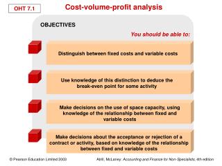
Understand the assumptions underlying cost-volume-profit (CVP) analysis. Learning Objective 1
Cost-Volume-Profit Assumptionsand Terminology 1. Changes in the level of revenues and costs arise only because of changes in the number of product (or service) units produced and sold. 2. Total costs can be divided into a fixed component and a component that is variable with respect to the level of output.
Cost-Volume-Profit Assumptionsand Terminology 3. When graphed, the behavior of total revenues and total costs is linear (straight-line) in relation to output units within the relevant range (and time period). 4. The unit selling price, unit variable costs, and fixed costs are known and constant.
Cost-Volume-Profit Assumptionsand Terminology 5. The analysis either covers a single product or assumes that the sales mix when multiple products are sold will remain constant as the level of total units sold changes. 6. All revenues and costs can be added and compared without taking into account the time value of money.
Cost-Volume-Profit Assumptionsand Terminology Operating income = Total revenues from operations – Cost of goods sold and operating costs (excluding income taxes) Net income = Operating income – Income taxes
Explain the features of CVP analysis. Learning Objective 2
Essentials of Cost-Volume-Profit(CVP) Analysis Example Assume that the Pants Shop can purchase pants for $32 from a local factory; other variable costs amount to $10 per unit. The local factory allows the Pants Shop to return all unsold pants and receive a full $32 refund per pair of pants within one year. The average selling price per pair of pants is $70 and total fixed costs amount to $84,000.
Essentials of Cost-Volume-Profit(CVP) Analysis Example How much revenue will the business receive if 2,500 units are sold? 2,500 × $70 = $175,000 How much variable costs will the business incur? 2,500 × $42 = $105,000 $175,000 – 105,000 – 84,000 = ($14,000)
Essentials of Cost-Volume-Profit(CVP) Analysis Example What is the contribution margin per unit? $70 – $42 = $28 contribution margin per unit What is the total contribution margin when 2,500 pairs of pants are sold? 2,500 × $28 = $70,000
Essentials of Cost-Volume-Profit(CVP) Analysis Example Contribution margin percentage (contribution margin ratio) is the contribution margin per unit divided by the selling price. What is the contribution margin percentage? $28 ÷ $70 = 40%
Essentials of Cost-Volume-Profit(CVP) Analysis Example If the business sells 3,000 pairs of pants, revenues will be $210,000 and contribution margin would equal 40% × $210,000 = $84,000.
Determine the breakeven point and output level needed to achieve a target operating income using the equation, contribution margin, and graph methods. Learning Objective 3
Breakeven Point Variable expenses Fixed expenses Sales – = Total revenues = Total costs
Abbreviations SP = Selling price VCU = Variable cost per unit CMU = Contribution margin per unit CM% = Contribution margin percentage FC = Fixed costs
Abbreviations Q = Quantity of output units sold (and manufactured) OI = Operating income TOI = Target operating income TNI = Target net income
Equation Method (Selling price × Quantity sold) – (Variable unit cost × Quantity sold) – Fixed costs = B/E in units Let Q = number of units to be sold to break even $70Q – $42Q – $84,000 = 0 $28Q = $84,000 Q = $84,000 ÷ $28 = 3,000 units
Contribution Margin Method (Fixed Costs ÷ CMU) = Breakeven point in units $84,000 ÷ $28 = 3,000 units Breakeven revenues = FC ÷ CM% $84,000 ÷ [(28 ÷ 70) x 100] = $210,000
Graph Method • Draw the Total Cost line • a. Start with the point at which the fixed cost intersects the vertical axis ($84,000 in our example) • b. Select a second point on the TC line. You need a second Q. For example, assume Q = 2,000. TC = 42Q + $84,000 . TC = 168,000. Plot this point on the graph. Extend a line horizontally from the first point in (a) above through the second point as now calculated. This is the TC line. • Draw the Total Revenue line • a. Begin with the point ‘0’ on the graph where the two axes intersect • b. Select a quantity (you may use the same as for TC) and compute TR. Plot point on the graph and extend a line from the (a) above through this new point on the graph. This is now your TR line
Graph Method Breakeven Revenue Total costs Fixed costs
Target Operating Income (Fixed costs + Target operating income) divided either by Contribution margin percentage or Contribution margin per unit
Target Operating Income Assume that management wants to have an operating income of $14,000. How many pairs of pants must be sold? Units to be sold = (Fixed Costs + Target Income) ÷ CMU ($84,000 + $14,000) ÷ $28 = 3,500 What dollar sales are needed to achieve this income? Revenue needed = (Fixed Costs + Target Income) ÷ CM% ($84,000 + $14,000) ÷ 40% = $245,000 ** Remember CM% = (Price – VC per unit) x 100**
Understand how income taxes affect CVP analysis. Learning Objective 4
Target Net Incomeand Income Taxes Example Management would like to earn an after tax income of $35,711. The tax rate is 30%. What is the target operating income? Target operating income = Target net income ÷ (1 – tax rate) TOI = $35,711 ÷ (1 – 0.30) = $51,016
Target Net Incomeand Income Taxes Example How many units must be sold? (FC + [Target Net Income ÷ (1 – Tax rate)]) CMU (84,000 + [35,711 ÷ (1- 0.3) ] ) (70 – 42) (84,000 + 51,016) ÷ $28 Q = $135,016 ÷ $28 = 4,822 pairs of pants
Target Net Incomeand Income Taxes Example Proof: Revenues: 4,822 × $70 $337,540 Variable costs: 4,822 × $42 202,524 Contribution margin $135,016 Fixed costs 84,000 Operating income 51,016 Income taxes: $51,016 × 30% 15,305 Net income $ 35,711
Explain CVP analysis in decision making and how sensitivity analysis helps managers cope with uncertainty. Learning Objective 5
Using CVP Analysis Example Suppose the management anticipates selling 3,200 pairs of pants. Management is considering an advertising campaign that would cost $10,000. It is anticipated that the advertising will increase sales to 4,000 units. Should the business advertise?
Using CVP Analysis Example 3,200 pairs of pants sold with no advertising: Contribution margin $89,600 Fixed costs 84,000 Operating income $ 5,600 4,000 pairs of pants sold with advertising: Contribution margin $112,000 Fixed costs 94,000 Operating income $ 18,000
Using CVP Analysis Example Instead of advertising, management is considering reducing the selling price to $61 per pair of pants. It is anticipated that this will increase sales to 4,500 units. Should management decrease the selling price per pair of pants to $61?
Using CVP Analysis Example 3,200 pairs of pants sold with no change in the selling price: Operating income = $5,600 4,500 pairs of pants sold at a reduced selling price: Contribution margin: (4,500 × $19) $85,500 Fixed costs 84,000 Operating income $ 1,500
Sensitivity Analysis andUncertainty Example Assume that the Pants Shop can sell 4,000 pairs of pants. Fixed costs are $84,000. Contribution margin ratio is 40%. At the present time the business cannot handle more than 3,500 pairs of pants.
Sensitivity Analysis andUncertainty Example To satisfy a demand for 4,000 pairs, management must acquire additional space for $6,000. Should the additional space be acquired? Revenues at breakeven with existing space are $84,000 ÷ .40 = $210,000. Revenues at breakeven with additional space are $90,000 ÷ .40 = $225,000
Sensitivity Analysis andUncertainty Example Operating income at $245,000 revenues with existing space = ($245,000 × .40) – $84,000 = $14,000. (3,500 pairs of pants × $28) – $84,000 = $14,000
Sensitivity Analysis andUncertainty Example Operating income at $280,000 revenues with additional space = ($280,000 × .40) – $90,000 = $22,000. (4,000 pairs of pants × $28 contribution margin) – $90,000 = $22,000
Use CVP analysis to plan fixed and variable costs. Learning Objective 6
Alternative Fixed/Variable CostStructures Example Suppose that the factory the Pants Shop is using to obtain the merchandise offers the following: Decrease the price they charge from $32 to $25 and charge an annual administrative fee of $30,000. What is the new contribution margin?
Alternative Fixed/Variable Cost Structures Example $70 – ($25 + $10) = $35 Contribution margin increases from $28 to $35. What is the contribution margin percentage? $35 ÷ $70 = 50% What are the new fixed costs? $84,000 + $30,000 = $114,000
Alternative Fixed/Variable Cost Structures Example Management questions what sales volume would yield an identical operating income regardless of the arrangement. 28x – 84,000 = 35x – 114,000 114,000 – 84,000 = 35x – 28x 7x = 30,000 x = 4,286 pairs of pants
Alternative Fixed/Variable Cost Structures Example Cost with existing arrangement = Cost with new arrangement .60x + 84,000 = .50x + 114,000 .10x = $30,000 x = $300,000 ($300,000 × .40) – $ 84,000 = $36,000 ($300,000 × .50) – $114,000 = $36,000
Apply CVP analysis to a company producing different products. Learning Objective 7
Effects of Sales Mix on Income Pants Shop Example Management expects to sell 2 shirts at $20 each for every pair of pants it sells. This will not require any additional fixed costs.
Effects of Sales Mix on Income Contribution margin per shirt: Price – VC per unit $20 – $9 = $11 What is the contribution margin of the mix? CMU for pants + CMU for shirts $28 + (2 × $11) = $28 + $22 = $50 *** The $28 is from the previous slides**
Effects of Sales Mix on Income $84,000 fixed costs ÷ $50 = 1,680 packages 1,680 × 2 = 3,360 shirts 1,680 × 1 = 1,680 pairs of pants Total units = 5,040
Effects of Sales Mix on Income What is the breakeven in dollars? 3,360 shirts × $20 = $ 67,200 1,680 pairs of pants × $70 = 117,600 $184,800
Effects of Sales Mix on Income What is the weighted-average budgeted contribution margin? Pants: 1 × $28 + Shirts: 2 × $11 = $50 ÷ 3 = $16.667
Effects of Sales Mix on Income The breakeven point for the two products is: $84,000 ÷ $16.667 = 5,040 units 5,040 × 1/3 = 1,680 pairs of pants 5,040 × 2/3 = 3,360 shirts
Effects of Sales Mix on Income Sales mix can be stated in sales dollars: PantsShirts Sales price $70 $40 Less: Variable costs 42 18 Contribution margin $28 $22 Contribution margin ratio 40% 55%
Effects of Sales Mix on Income Now, let’s assume the sales mix in dollars is 63.6% pants and 36.4% shirts. Weighted contribution would be: 40% × 63.6% = 25.44% pants 55% × 36.4% = 20.02% shirts 45.46%
Effects of Sales Mix on Income Breakeven sales dollars is $84,000 ÷ 45.46% = $184,778 (rounding). $184,778 × 63.6% = $117,519 pants sales $184,778 × 36.4% = $ 67,259 shirt sales