Download
1 / 9
150 likes | 538 Vues
Ch. 53 Exponential and Logistic Growth. Objective: SWBAT explain how competition for resources limits exponential growth and can be described by the logistic growth model. Exponential Growth. Unrealistic! Does not take into account limiting factors (resources and competition).

E N D
Ch. 53 Exponential and Logistic Growth Objective: SWBAT explain how competition for resources limits exponential growth and can be described by the logistic growth model.
Exponential Growth • Unrealistic! Does not take into account limiting factors (resourcesand competition). • However, a good model for showing upper limits of growth and conditions that would facilitate growth.
Change in population size Immigrants entering population Emigrants leaving population Births Deaths dN rmaxN dt N rN t Exponential Growth Equation Per capita (individual) B bN D mN Per capita growth rate r b m Under ideal conditions, growth rate is at its max
2,000 Exponential Graph dNdt = 1.0N 1,500 dNdt = 0.5N • Exponential growth results in a J curve. Population size (N) 1,000 500 0 5 10 15 Number of generations
Real Life Examples 8,000 6,000 • Can occur when: • Populations move to a new area. • Rebounding after catastrophic event (Cambrian explosion) Elephant population 4,000 2,000 0 1900 1910 1920 1930 1940 1950 1960 1970 Year
Logistic Growth • Takes into account limiting factors. More realistic. • Population size increases until a carrying capacity (K) is reached (then growth decreases as pop. size increases). • point at which resources and population size are in equilibrium. • K can change over time (seasons, pred/prey movements, catastrophes, etc.).
(K N) dN rmax N dt K Logistic Growth Equation
Exponentialgrowth Logistic Graph 2,000 dN dt = 1.0N 1,500 • Logistic growth results in an S-shaped curve K = 1,500 Logistic growth 1,500 – N 1,500 dN dt ( ) Population size (N) = 1.0N 1,000 Population growthbegins slowing here. 500 0 0 5 10 15 Number of generations
Real Life Examples Note overshoot 180 1,000 150 800 120 Number of Daphnia/50 mL Number of Paramecium/mL 600 90 400 60 200 30 0 0 0 5 10 15 0 20 40 60 80 100 120 140 160 Time (days) Time (days) (b) A Daphnia population in the lab (a) A Paramecium population in the lab