Understanding Magnetic Switching: Spin Wave Visualization
Understanding Magnetic Switching: Spin Wave Visualization. P. B.Visscher, D. M. Apalkov, and X.Feng Department of Physics and Astronomy The University of Alabama. Web version.

Understanding Magnetic Switching: Spin Wave Visualization
E N D
Presentation Transcript
Understanding Magnetic Switching: Spin Wave Visualization P. B.Visscher, D. M. Apalkov, and X.Feng Department of Physics and Astronomy The University of Alabama Web version Movies will not play until they’ve been downloaded and correctly pointed to – it may be easier to play them from the web page (folder directory) directly. They have names like HUp.mov, HDown.mov, HHor.mov, OneCell Hz=Hk.mov, etc. Narration is in notes (icon on lower left toolbar will give the notes window)|
Curling M • Buckling • Nucleation at end Motivation We want to understand switching in magnetic media (e.g., hard disk). Basic problem: switch Known mechanisms: to M
OR, spin-wave switching (Safonov & Bertram 1999): Movie 1Initial motion, just after reversing external field. See precession about field, then “breakup”.
Switching Simulation • Magnetization vs time for a 4 4 4 system: Movie 2 Movie 1
Movie 2After system has halfway switched from up to down. Lots of spin wave energy.
Basic equation for precession • Landau-Lifshitz equation without • damping (not important in early stages of fast switching) • thermal (Langevin) noise (small, kBT<<Zeeman energy)
We want to switch the magnetization so it points down -- try reversing magnetic field H from up to down:
Precessional switching Since M precesses around H, the way to get M to swing down is to use a horizontal H:
Anisotropy field (due to intrinsic crystalline anisotropy or to sample shape)
Add a vertical component to Hext to cancel anisotropy field:
Decrease Hext so it doesn’t quite cancel HK. Then precession around z has both signs, tends to cancel.
Spin waves A homogeneous system can get near the “hard plane” but it will always come back (closed orbits). In spin wave switching simulations we saw inhomogeneity: spin waves. To understand spin waves we have to introduce exchange interactions: Neighboring spins (or magnetized finite elements) exert exchange fields on each other: If all M’s are parallel the exchange field has no effect (MxH=0). But if they aren’t, M’s precess around each other (spin waves). M M’ Hexch
One spin wave ?? spin waves
Visualizing spin waves Fourier-transform to get spin wave amplitudes: Each M(r) can be written as the sum of its Fourier components: where the Fourier component is Rather than display the complex vector M(k), we display all the individual components Mk(r) for all cells r. (N vectors, not N3.)
Back to switching We found that a uniform system with an almost-downward H would get close to the equator, but not switch. Add exchange interactions (spin waves):
Why is it unstable?Calculating (FMR) precession frequency General formula for spin-wave frequency (=resonance frequency for FMR, if k=0) where DM is the demag+anisotropy factor along M and Dt1 and Dt2 are demag+anisotropy factors transverse to M • In the simple case of M along the easy (z) axis, DM =2K/Ms and Dt1 = Dt2 = 0, so w2 > 0 and w is real: we get circular precession. • If M is along a hard axis, Dt1 = 2K/Ms and one factor can be negative, making w imaginary (exponentially growing instability). This is the origin of the switching instability.
History of hard-plane FMR Oddly enough, this instability was known experimentally as early as 1955. Along a hard axis, the frequency becomes As we lower the hard axis field H, this vanishes at a critical value Hc = 2K/Ms. Below Hc, M will not remain along the hard axis, so we cannot do FMR. J. Smit and H. G. Beljers, Phillips Res. Rept.10, 113 (1955), reproduced from “The Physical Principles of Magnetism”, A. H. Morrish, 1965.
Simulation of simple hard-plane instability Below Hc = 2K/Ms, M will not remain along the hard axis, so we cannot do FMR, but we can do a short-time simulation:
Back to switching We found that a uniform system with an almost-downward H would get close to the equator, but not switch. Add exchange interactions (spin waves):
Summary • We have identified the instability responsible for spin wave switching. Remaining to do: • Consider samples with boundaries (everything here was with periodic b.c.’s) • Add magnetostatic interactions (Fast Multipole Method) • Determine which wavelengths are most unstable
Why perpendicular recording? Longitudinal Perpendicular-recording head Longitudinal N S medium Smaller write field in longitudinal case Larger write field in perpendicular case