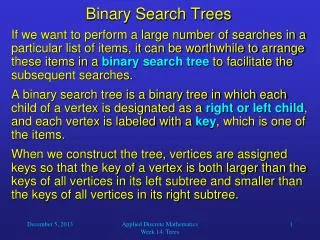
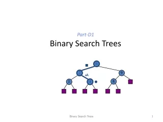
Part-D1 Binary Search Trees

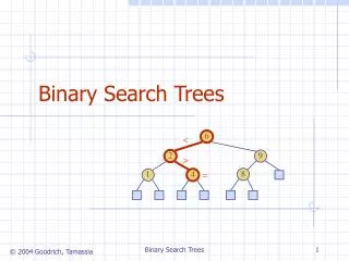
1. Part-D1Binary Search Trees 6 < 2 9 > = 8 1 4 Binary Search Trees

2. Binary Search (§ 8.3.3) • Binary search can perform operation find(k) on a dictionary implemented by means of an array-based sequence, sorted by key • at each step, the number of candidate items is halved • terminates after O(log n) steps • Example: find(7) 0 1 3 4 5 7 8 9 11 14 16 18 19 m h l 0 1 3 4 5 7 8 9 11 14 16 18 19 m h l 0 1 3 4 5 7 8 9 11 14 16 18 19 m h l 0 1 3 4 5 7 8 9 11 14 16 18 19 l=m =h Binary Search Trees

3. 6 2 9 1 4 8 Binary Search Trees (§ 10.1) • A binary search tree is a binary tree storing keys (or key-value entries) at its internal nodes and satisfying the following property: • Let u, v, and w be three nodes such that u is in the left subtree of v and w is in the right subtree of v. We have key(u)key(v) key(w) • External nodes do not store items • An inorder traversal of a binary search trees visits the keys in increasing order Binary Search Trees

4. Search (§ 10.1.1) AlgorithmTreeSearch(k, v) ifT.isExternal (v) returnv if k<key(v) returnTreeSearch(k, T.left(v)) else if k=key(v) returnv else{ k>key(v) } returnTreeSearch(k, T.right(v)) • To search for a key k, we trace a downward path starting at the root • The next node visited depends on the outcome of the comparison of k with the key of the current node • If we reach a leaf, the key is not found and we return null • Example: find(4): • Call TreeSearch(4,root) 6 < 2 9 > = 8 1 4 Binary Search Trees

5. Insertion 6 < • To perform operation insert(k, o), we search for key k (using TreeSearch) • Assume k is not already in the tree, and let w be the leaf reached by the search • We insert k at node w and expand w into an internal node • Example: insert 5 2 9 > 1 4 8 > w 6 2 9 1 4 8 w 5 Binary Search Trees

6. Insertion 6 < • To perform operation insert(k, o), we search for key k (using TreeSearch) Algorithm TreeINsert(k, x, v): Input: A search key, an associate value x and a node v of T to start with Output: a new node w in the subtree T(v) that stores the entry (k, x) W TreeSearch(k,v) If k=key(w) then return TreeInsert(k, x, T.left(w)) T.insertAtExternal(w, (k, x)) Return • Example: insert 5 • Example: insert another 5? 2 9 > 1 4 8 > w 6 2 9 1 4 8 w 5 Binary Search Trees

7. Deletion • To perform operation remove(k), we search for key k • Assume key k is in the tree, and let v be the node storing k • If node v has a leaf child w, we remove v and w from the tree with operation removeExternal(w), which removes w and its parent • Example: remove 4 6 < 2 9 > v 1 4 8 w 5 6 2 9 1 5 8 Binary Search Trees

8. Deletion (cont.) 1 • We consider the case where the key k to be removed is stored at a node v whose children are both internal • we find the internal node w that follows v in an inorder traversal • we copy key(w) into node v • we remove node w and its left child z (which must be a leaf) by means of operation removeExternal(z) • Example: remove 3 v 3 2 8 6 9 w 5 z 1 v 5 2 8 6 9 Binary Search Trees

9. Deletion (Another Example) 1 v 3 2 8 6 9 w 4 z 5 1 v 4 2 8 6 9 5 Binary Search Trees

10. Performance • Consider a dictionary with n items implemented by means of a binary search tree of height h • the space used is O(n) • methods find, insert and remove take O(h) time • The height h is O(n) in the worst case and O(log n) in the best case Later, we will try to keep h =O(log n). Binary Search Trees

11. 6 v 8 3 z 4 AVL Trees AVL Trees

12. AVL Tree Definition • AVL trees are balanced. • An AVL Tree is a binary search tree such that for every internal node v of T, the heights of the children of v can differ by at most 1. An example of an AVL tree where the heights are shown next to the nodes: AVL Trees

13. 6 4 8 5 1 7 11 AVL tree 3 6 4 8 1 5 7 11 3 not an AVL tree 2 TCSS 342 AVL Trees v1.0

14. AVL Tree -1 0 0 0 -1 1 0 0 0 0 AVL Tree -2 AVL Tree 1 0 0 -1 0 Not an AVL Tree

15. n(2) 3 n(1) 4 Height of an AVL Tree • Fact: The height of an AVL tree storing n keys is O(log n). • Proof: Let us bound n(h): the minimum number of internal nodes of an AVL tree of height h. • We easily see that n(1) = 1 and n(2) = 2 • For n > 2, an AVL tree of height h contains the root node, one AVL subtree of height n-1 and another of height n-2 (or n-1). • That is, n(h)  1 + n(h-1) + n(h-2) • Knowing n(h-1) > n(h-2), we get n(h) > 2n(h-2). So n(h) > 2n(h-2), n(h) > 4n(h-4), n(h) > 8n(h-6), … (by induction), n(h) > 2in(h-2i) • Solving the base case we get: n(h) > 2 (h/2)-1 • Taking logarithms: h < 2log n(h) +2 • Thus the height of an AVL tree is O(log n) AVL Trees

16. 44 17 78 44 32 50 88 17 78 48 62 32 50 88 54 48 62 Insertion in an AVL Tree • Insertion is as in a binary search tree • Always done by expanding an external node. • Example: c=z a=y b=x w before insertion after insertion AVL Trees

17. Names of important nodes • w: the newly inserted node. (insertion process follow the binary search tree method) • The heights of some nodes in T might be increased after inserting a node. • Those nodes must be on the path from w to the root. • Other nodes are not effected. • z: the first node we encounter in going up from w toward the root such that z is unbalanced. • y: the child of z with higher height. • y must be an ancestor of w. (why? Because z in unbalanced after inserting w) • x: the child of y with higher height. • x must be an ancestor of w. • The height of the sibling of x is smaller than that of x. (Otherwise, the height of y cannot be increased.) • See the figure in the last slide. Binary Search Trees

18. Algorithm restructure(x): Input: A node x of a binary search tree T that has both parent y and grand-parent z. Output: Tree T after a trinode restructuring. • Let (a, b, c) be the list (increasing order) of nodes x, y, and z. Let T0, T1, T2 T3 be a left-to-right (inorder) listing of the four subtrees of x, y, and z not rooted at x, y, or z. • Replace the subtree rooted at z with a new subtree rooted at b.. • Let a be the left child of b and let T0 and T1 be the left and right subtrees of a, respectively. • Let c be the right child of b and let T2 and T3 be the left and right subtrees of c, respectively. Binary Search Trees

19. c = z b = y single rotation b = y a = x c = z a = x T T 3 0 T T T T T 0 2 1 2 3 T 1 Restructuring (as Single Rotations) • Single Rotations: Binary Search Trees

20. double rotation c = z b = x a = y a = y c = z b = x T T 3 1 T T T T T 0 0 2 3 1 T 2 Restructuring (as Double Rotations) • double rotations: Binary Search Trees

21. T T 1 1 Insertion Example, continued unbalanced... 4 44 x 3 2 17 62 z y 2 1 2 78 32 50 1 1 1 ...balanced 54 88 48 T 2 T T AVL Trees 0 3

22. Theorem: • One restructure operation is enough to ensure that the whole tree is balanced. • Proof: Look at the four cases on slides 20 and 21. After restructure operation, the height of the sub-tree is reduced by one. Binary Search Trees

23. 44 17 62 32 50 78 88 48 54 Removal in an AVL Tree • Removal begins as in a binary search tree by calling removal(k) for binary tree. • may cause an imbalance. • Example: 44 w 17 62 50 78 88 48 54 before deletion of 32 after deletion Binary Search Trees

24. Rebalancing after a Removal • Let z be the first unbalanced node encountered while travelling up the tree from w. w-parent of the removednode (in terms of structure, not the name. See Slide 12-14) • let y be the child of z with the larger height, • let x be the child of y defined as follows; • If one of the children of y is taller than the other, choose x as the taller child of y. • If both children of y have the same height, select x be the child of y on the same side as y (i.e., if y is the left child of z, then x is the left child of y; and if y is the right child of z then x is the right child of y.) • The way to obtain x, y and z are different from insertion. Binary Search Trees

25. Rebalancing after a Removal • We perform restructure(x) to restore balance at z. • As this restructuring may upset the balance of another node higher in the tree, we must continue checking for balance until the root of T is reached 62 44 a=z 44 78 w 17 62 b=y 17 50 88 50 78 c=x 48 54 88 48 54 Binary Search Trees

26. Unbalanced after restructuring Unbalanced balanced 1 1 62 h=3 44 h=4 h=5 a=z h=5 44 78 17 62 w b=y 17 50 88 32 50 78 c=x 88 Binary Search Trees

27. Rebalancing after a Removal • We perform restructure(x) to restore balance at z. • As this restructuring may upset the balance of another node higher in the tree, we must continue checking for balance until the root of T is reached 62 44 a=z 44 78 17 62 w b=y 17 50 88 50 78 c=x 48 54 88 48 54 Binary Search Trees

28. 44 17 62 32 50 78 88 48 54 Example a: • Which node is w? Let us remove node 17. 44 w 32 62 50 78 88 48 54 before deletion of 32 after deletion Binary Search Trees

29. Rebalancing: • We perform restructure(x) to restore balance at z. • As this restructuring may upset the balance of another node higher in the tree, we must continue checking for balance until the root of T is reached 62 44 a=z 44 78 w 32 62 b=y 32 50 88 50 78 c=x 48 54 88 48 54 Binary Search Trees

30. Running Times for AVL Trees • a single restructure is O(1) • using a linked-structure binary tree • find is O(log n) • height of tree is O(log n), no restructures needed • insert is O(log n) • initial find is O(log n) • Restructuring up the tree, maintaining heights is O(log n) • remove is O(log n) • initial find is O(log n) • Restructuring up the tree, maintaining heights is O(log n) AVL Trees