4 .5 Basic Parameters for Audio Analysis

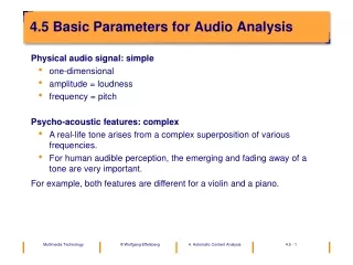
1. Physical audio signal: simple • one-dimensional • amplitude = loudness • frequency = pitch • Psycho-acoustic features: complex • A real-life tone arises from a complex superposition of various frequencies. • For human audible perception, the emerging and fading away of a tone are very important. • For example, both features are different for a violin and a piano. 4.5 Basic Parameters for Audio Analysis

2. Perception of Loudness • The physical measure is called acoustic pressure, the unit is decibel (dB-SPL, Sound Pressure Level). • The human audible perception is called loudness, the unit is phon. • We can empirically derive a set of curves that depicts the perceived loudness as a function of acoustic pressure and frequency. They are called isophones.

3. Experimental Results • red curve: acoustic pressure • black curve: loudness as perceived by test subjects • blue curve: computationally predicted perceived loudness

4. Fundamental Frequencies in Harmonic Sounds • The period of the composite tone f0 corresponds to the least common multiple of the periods of the two composing frequencies f1 and f2.

5. Frequency Transformations • J.B.J. Fourier (1768-1830): Each periodic oscillation can be written as the sum of harmonic frequencies: f: frequency Af,Bf: amplitudes

6. Frequency Transformation of an Audio Signal Steps 3 and 4 can be sped up considerably by means of the Fast Fourier transform (FFT). The complexity of FFT is O(n log n) compared to O(n2).

7. Time domain Frequency domain Step 1: Sampling in the Time Domain

8. Time domain Frequency domain Step 2: Time Restriction to [0, NT]

9. Time domain Frequency domain Step 3: Sampling in the Frequency Domain • Goal: Discretization of the data also in the frequency domain (for representation in the computer) Reference: E.Oran Brigham: Fast Fourier Transform and Its Applications, Prentice Hall, 1997

10. Signal Analysis with the DFT • Assumption • A natural audio signal of sampling length M is given, e.g., M = 5minof music. • Goal • Extraction of features, e.g., musical tones (pitch, loudness, onset, etc.) • Method • Definition of a window of size N which is moved over the audio signal. It represents a window of analysis. The DFT is computed on this window. Only with a windowed DFT, we can analyze the behavior of the signal over time. • Example: We can assume that musical tones are stationary for at least 10 ms. We thus choose N = 10 ms. When moving the window, we allow redundancy in order to also analyze the transitions between tones. Here, we chose an overlap of 2 ms. This results in frames.

11. Signal Analysis – Properties (1) • It is now possible to compute semantic features for the sample frames. • 1. Energy m = ending time of the frame Es is a measure for the acoustic energy of the signal in the frame. It cor-responds to the square of the area under the curve in the time domain. The energy might as well be computed for the frequency-transformed sig-nal. It then denotes a measure for its spectral energy spread. Computing the energy in the frequency space makes sense if one is interested in knowing frequency ranges in which the energy occurs.

12. Signal Analysis – Properties (2) • 2. Zero-crossings • Counts the number of zero-crossings (i.e., sign changes) of the signal. • High frequencies lead to a high Zs while low frequencies lead to a low Zs • This is closely related to the basic frequencies contained in the signal. • Many other parameters are also used in audio signal analysis.