Download
1 / 25
250 likes | 393 Vues
A Tractable Pseudo-Likelihood for Bayes Nets Applied To Relational Data. Oliver Schulte School of Computing Science Simon Fraser University Vancouver, Canada. Machine Learning for Relational Databases. Typical SRL Tasks

E N D
A Tractable Pseudo-Likelihood for Bayes Nets Applied To Relational Data • Oliver Schulte • School of Computing Science • Simon Fraser University • Vancouver, Canada
Machine Learning for Relational Databases Typical SRL Tasks • Link-based Classification: predict the class label of a target entity,given the links of a target entity and the attributes of related entities. • Link Prediction: predict the existence of a link,given the attributes of entities and their other links. • Generative Modelling: represent the joint distribution over links and attributes. • Relational Databases dominate in practice. • Want to apply Machine Learning Statistical-Relational Learning. • Fundamental issue: how to combine logic and probability? ★Today Pseudo-Likelihood for Relational Data - SDM '11
Measuring Model Fit Statistical Learning requires a quantitative measure of data fit. e.g., BIC, AIC: log-likelihood of data given model + complexity penalty. • In relational data, units are interdependent • no product likelihood function for model. • Proposal of this talk: use pseudo likelihood. • Unnormalized product likelihood. • Like independent-unit likelihood, but with event frequencies instead of event counts. Pseudo-Likelihood for Relational Data – SIAM ‘11
Outline • Relational databases. • Bayes Nets for Relational Data (Poole IJCAI 2003). • Pseudo-likelihood function for 1+2. • Random Selection Semantics. • Parameter Learning. • Structure Learning. Pseudo-Likelihood for Relational Data - SDM '11
Database Instance based on Entity-Relationship (ER) Model Key fields are underlined.Nonkey fields are deterministic functions of key fields. Pseudo-Likelihood for Relational Data - SDM '11
Relational Data: what are the random variables (nodes)? • A functor is a function or predicate symbol (Prolog). • A functor random variable is a functor with 1st-order variables f(X), g(X,Y), R(X,Y). • Each variable X,Y,… ranges over a population or domain. • A FunctorBayes Net* (FBN) is a Bayes Net whose nodes are functor random variables. • Highly expressive (Domingos and Richardson MLJ 2006, Getoor and Grant MLJ 2006). *David Poole, “First-Order Probabilistic Inference”, IJCAI 2003. Originally: ParametrizedBayes Net. Pseudo-Likelihood for Relational Data - SDM '11
Example: Functor Bayes Nets =T =T =T =T =F =T =T • Parameters: conditional probabilities P(child|parents). • Defines joint probability for every conjunction of value assignments. What is the interpretation of the joint probability? Pseudo-Likelihood for Relational Data - SDM '11
Random Selection Semantics of Functors • Intuitively, P(Flies(X)|Bird(X)) = 90% means “the probability that a randomly chosen bird flies is 90%”. • Think of X as a random variable that selects a member of its associated population with uniform probability. • Nodes like f(X), g(X,Y) are functions of random variables, hence themselves random variables. Halpern, “An analysis of first-order logics of probability”, AI Journal 1990.Bacchus, “Representing and reasoning with probabilistic knowledge”, MIT Press 1990. Pseudo-Likelihood for Relational Data - SDM '11
Random Selection Semantics: Examples Users • P(X = Anna) = 1/2. • P(Smokes(X) = T) = x:Smokes(x)=T 1/|X| = 1. • P(Friend(X,Y) = T) = x,y:Friend(x,y) 1/(|X||Y|). • The database frequency of a functor assignment is the number of satisfying instantiations or groundings, divided by the total possible number of groundings. Friend Pseudo-Likelihood for Relational Data - SDM '11
Likelihood Function for Single-Table Data =T =F =T Smokes(Y) Cancer(Y) decomposed (local) data log-likelihood Users Table T count of co-occurrences of child node value and parent state Parameter of Bayes net B Likelihood/Log-likelihood Pseudo-Likelihood for Relational Data - SDM '11
Proposed Pseudo Log-Likelihood =T =T For database D: Smokes(X) Friend(X,Y) Smokes(Y) Cancer(Y) =T Users Database D frequency ofco-occurrences of child node value and parent state Parameter of Bayes net Friend Pseudo-Likelihood for Relational Data - SDM '11
Semantics: Random Selection Log-Likelihood • Randomly select instances X1 = x1,…,Xn=xn for each variable in FBN. • Look up their properties, relationships in database. • Compute log-likelihood for the FBN assignment obtained from the instances. • LR = expected log-likelihood over uniform random selection of instances. Smokes(X) Friend(X,Y) Smokes(Y) Cancer(Y) LR = -(2.254+1.406+1.338+2.185)/4 ≈ -1.8 Proposition The random selection log-likelihood equals the pseudo log-likelihood. Pseudo-Likelihood for Relational Data - SDM '11
Parameter Learning Is Tractable Proposition For a given database D, the parameter values that maximize the pseudo likelihood are the empirical conditional frequencies in the database. Pseudo-Likelihood for Relational Data - SDM '11
Structure Learning • In principle, just replace single-table likelihood by pseudo likelihood. • Efficient new algorithm (Khosravi, Schulte et al. AAAI 2010). Key ideas: • Use single-table BN learner as black box module. • Level-wise search through table join lattice. Results from shorter paths are propagated to longer paths (think APRIORI). Pseudo-Likelihood for Relational Data - SDM '11
Running time on benchmarks • Time in Minutes. NT = did not terminate. • x + y = structure learning + parametrization (with Markov net methods). • JBN: Our join-based algorithm. • MLN, CMLN: standard programs from the U of Washington (Alchemy) Pseudo-Likelihood for Relational Data - SDM '11
Accuracy • Inference: use MLN algorithm after moralizing. • Task (Kok and Domingos ICML 2005): • remove one fact from database, predict given all others. • report average accuracy over all facts. Pseudo-Likelihood for Relational Data - SDM '11
Summary: Likelihood for relational data. • Combining relational databases and statistics. • Very important in practice. • Combine logic and probability. • Interdependent units hard to define model likelihood. • Proposal: Consider a randomly selected small group of individuals. • Pseudo log-likelihood = expected log-likelihood of randomly selected group. Pseudo-Likelihood for Relational Data - SDM '11
Summary: Statistics with Pseudo-Likelihood • Theorem: Random pseudo log-likelihood equivalent to standard single-table likelihood, replacing table counts with database frequencies. • Maximum likelihood estimates = database frequencies. • Efficient Model Selection Algorithm based on lattice search. • In simulations, very fast (minutes vs. days), much better predictive accuracy. Pseudo-Likelihood for Relational Data - SDM '11
Thank you! • Any questions? Pseudo-Likelihood for Relational Data - SDM '11
Comparison With Markov Logic Networks (MLNs) Friend(X,Y) Smokes(X) Smokes(Y) Cancer(Y) • MLNs are basically undirected graphs with functor nodes. One of the most successful statistical-relational formalisms. • ln P(D|MBN) • Let MBN = Bayes net converted to MLN. • Log-likelihood of MBN = pseudo log-likelihood of B + normalization constant. Friend(X,Y) Smokes(X) Smokes(Y) Cancer(Y) • ln P*(D|BN) • ln(P(D|MBN) = ln P*(D|BN) + ln(Z) “Markov Logic: An Interface Layer for Artificial Intelligence”. Domingos and Lowd 2009.
Likelihood Functions for Parametrized Bayes Nets • Problem: Given a database D and an FBN model B, how to define model likelihood P(D|B)? • Fundamental Issue: interdependent units, not iid. • Previous approaches: • Introduce latent variables such that units are independent conditional on hidden “state” (e.g., Kersting et al. IJCAI 2009). • Different model class, computationally demanding. • Related to nonnegative matrix factorization----Netflix challenge. • Grounding, or Knowledge-based Model Construction (Ngo and Haddaway, 1997; Koller and Pfeffer, 1997; Haddaway, 1999; Poole 2003). • Can lead to cyclic graphs. • Undirected models (Taskar, Abeel, Koller UAI 2002, Domingos and Richardson ML 2006). Pseudo-Likelihood for Relational Data - SDM '11
Hidden Variables Avoid Cycles U(X) U(Y) Rich(X) Friend(X,Y) Rich(Y) • Assign unobserved values u(jack), u(jane). • Probability that Jack and Jane are friends depends on their unobserved “type”. • In ground model, rich(jack) and rich(jane) are correlated given that they are friends, but neither is an ancestor. • Common in social network analysis (Hoff 2001, Hoff and Rafferty 2003, Fienberg 2009). • $1M prize in Netflix challenge. • Also for multiple types of relationships (Kersting et al. 2009). • Computationally demanding. Causal Modelling for Relational Data - CFE 2010
The Cyclicity Problem Friend(X,Y) Rich(X) Class-level model (template) Rich(Y) Rich(a) Friend(a,b) Friend(b,c) Friend(c,a) Ground model Rich(b) Rich(c) Rich(a) • With recursive relationships, get cycles in ground model even if none in 1st-order model. • Jensen and Neville 2007: “The acyclicity constraints of directed models severely constrain their applicability to relational data.” Causal Modelling for Relational Data - CFE 2010
Undirected Models Avoid Cycles Friend(X,Y) Rich(X) Class-level model (template) Rich(Y) Friend(a,b) Friend(c,a) Friend(b,c) Ground model Rich(a) Rich(b) Rich(c) Causal Modelling for Relational Data - CFE 2010
Choice of Functors • Can have complex functors, e.g. • Nested: wealth(father(father(X))). • Aggregate: AVGC{grade(S,C): Registered(S,C)}. • In remainder of this talk, use functors corresponding to • Attributes (columns), e.g., intelligence(S), grade(S,C) • Boolean Relationship indicators, e.g. Friend(X,Y). Pseudo-Likelihood for Relational Data - SDM '11