Remediation of Enhanced Radiation Belts: Insights from Low Latitude Wave Injection Research
130 likes | 272 Vues
This workshop report discusses the findings from experiments on wave injection at low latitudes, specifically targeting enhanced radiation belts using a navigation transmitter in Komsomolsk na Amur. The study includes data from Stanford University receivers and aims to quantify wave growth and propagation characteristics related to geomagnetic activity. Over a 10-day observation period, temporal growth rates of 70-80 dB/sec were recorded, along with diurnal patterns correlating with geomagnetic disturbances. Future work will focus on quantifying the relationship between these waves and geomagnetic conditions.

Remediation of Enhanced Radiation Belts: Insights from Low Latitude Wave Injection Research
E N D
Presentation Transcript
Wave Injection at Low Latitudes Mark Golkowski Remediation of Enhanced Radiation Belts Workshop Lake Arrowhead, CA March 3-6, 2007
Adelaide, Australia • ~500 kW ? Navigation transmitter in Komsomolsk na Amur in Russian far east (400 msec pulses) at L = 2 • Conjugate point in southern Australia • Stanford University receiver since January 2007 • Explore and quantify wave-growth Stanford Scientists Kangaroos
Russian Alpha Transmitters • 3.6 second pattern (six 0.6s segments) • 400ms pulses, 200ms off between pulses • Three sites alternate among 3 frequencies 14.88 kHz
Historical Background • Triggered emissions have been observed from other mid-latitude transmitters: NAA (L=2) 14.5 kHz, 200 msec pulses • Whistler-mode Komsomolsk Alpha pulses have been studied by Tanaka et al. 1987 in the context of whistler propagation characteristics
Example Growth ~7-8 dB total ~70-80 dB/sec
10-Day Statistics (1-10 April) • Count of 1-hop observations in synoptic (1min/5min) recordings • 10 days during and after a geomagnetic disturbance • 1-Hop observations show qualitative relationship to geomagnetic activity Need more data to quantify relationship
Diurnal patterns Day Night Day Day Night Day
Average Daily Variations Tanaka et al. 1987 Stanford 2008 Sunset Sunrise • Diurnal variation shows maxima after sunset and sunrise • Tanaka et al. 1987: diurnal variation is same for whistlers and is a propagation effect (duct formation, coupling in/out of duct)
Summary • 1-Hop echoes regularly observed from Komsomolsk Alpha transmitter • Echoes exhibit temporal growth of ~70-80 dB/sec • Propagation delays of 460 msec – 540msec equatorial electron concentrations of 4000-5000 cm-3 at L = 2 • Triggered of frequency emmisions not observed yet, except perhaps on DEMETER satellite • Diurnal variations likely result from propagation/ducting effects • Future Work: statistically quantify effect of geomagnetic conditions on wave growth