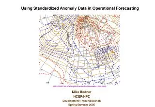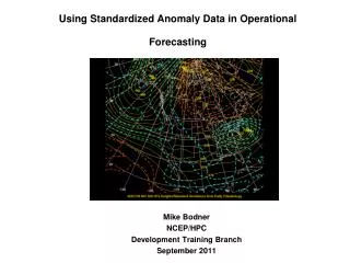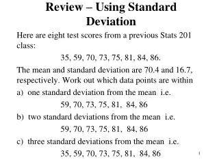
Using Standard Deviation Data in Operational Forecasting
Using Standard Deviation Data in Operational Forecasting. Mike Bodner NCEP/HPC Development Training Branch Fall 2004. Outline. Overview of standard deviations and statistical methods in forecasting Methodology and computational information behind operational standard deviations

Using Standard Deviation Data in Operational Forecasting
E N D
Presentation Transcript
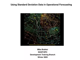
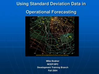
Using Standard Deviation Data in Operational Forecasting Mike Bodner NCEP/HPC Development Training Branch Fall 2004
Outline • Overview of standard deviations and statistical methods in forecasting • Methodology and computational information behind operational standard deviations • Application of standard deviations • Look at significant cases
We are already using tools that apply stochastic methods in operational forecasting… • MOS output • Ensembles • SREFs
Standard deviations can be another tool to add to the chest… • Based on 50 years of climatology • Can be applied to a model forecast output • Fields can be compared to record breaking or extreme events from past dates • Can help discern how whether or not model forecast is way off the mark or not
How are standard deviations generated? • Daily averages and variance are computed for 500 hPa heights and 850 hPa temperatures from NCAR/NCEP Reanalysis data from 1950-2001 Variance is the mean or expected value of the squared deviations from the mean itself or by the expression var(x) = MEAN{[x-MEAN(x)]**2}
Another way of looking at it using 500 hPa heights… Standard deviation or σ is computed by the following formula.. σ= square root of the average of heights 2 - average height2 The number of standard deviations from the climatology is computed by subtracting the 50 year average height from the model forecast or observed height then dividing by the standard deviation. # of standard deviations = (fcst height - average height) ÷ σ
Keep in mind when looking at standard deviation data in an operational setting.. • Whenever the models are forecasting the number of standard deviations to be 3 units of more from climatology, a significant or extraordinary event is being suggested • A record breaking temperature or precipitation scenario is possible • Typically 3-4 standard deviations from normal during the cold season and 2-3 in the warm season • Forecast values of 5 and 6 are of extremely low probability and should be closely scrutinized if displayed in model forecast data
Surprise October 1996 snow event in Kansas City metro area..4 SDs lower than climatology
Other items to be aware of when using this tool • It’s beneficial to be aware of the standard deviations or at least the SD pattern for your forecast data • The climatological standard deviations are not as large over the southern latitudes, particularly during the warm season • The probability of the heights and temperatures do not follow a normal distribution in southern and tropical latitudes where heights or temperatures are more likely to exceed 1 standard deviation
Here’s an example of the computed standard deviations for 500 hPa heights forJuly 4. Notice how the variance increases proportionally with latitude. Also note how the largest variance occurs over the North Pacific and North Atlantic.
Let’s apply the SD data from the July 4 image in the previous slide… • At Atlanta, GA. The average 500 hPa height for July 4 is 588 dm, and the standard deviation for 500 hPa height over Atlanta is 3 dm • A forecast value of 3 standard deviationsfrom normal or -3 would suggest a forecast height of 579 dm which is 9 dm below climatology • At Seattle, WA. The average 500 hPa height for July 4 is about 570 dm, and the standard deviation for 500 hPa height over Seattle is 9 dm • A forecast value of 3 standard deviationsfrom normal or -3 would suggest a forecast height of 543 dm or 27 dm below climatology.
As mentioned several slides earlier, height and temperature regimes depicted as 3 or more standard deviations from climatology are very rare. The number of standard deviations are displayed with probability of occurrence of the number of standard deviations from climatology based on a standard probability density function (PDF) curve. The values include both above and below normal conditions.
The values plotted on the standard "bell curve" depict percent probability of a standard deviation being above or below the climatological mean (essentially these values are half of the probabilities sited in the above chart). As you can see, there is extremely low probability for forecast events greater than 3 standard deviations from climatology.
Let’s take a look a few regional heat cases… • Northeast U.S. Heat Wave – July 1966 • Central U.S. Heat Wave – July 1980 • Southwest U.S. Extreme Heat – June 1990
4th of July Heat Wave over the Northeast U.S. Triple digit temperatures were noted over many Northeast locations during the 3 day period 3-5 July 1966. The 500 hPa charts for this record breaking heat event over the Northeast do not depict a pattern typical of a severe heat wave. 500 hPa heights are 2 standard deviations above climatology but the next slide depicts the 850 hPa thermal field which ended up being the driver in this pattern.
850 hPa temperatures and standard deviations The high 850 temperatures were 2.5 standard deviations above normal. The anomalously warm thermal field coupled with down sloping were primary contributors to the record breaking heat of 3-5 July, 1966.
Central U.S. Heat Wave 1980 A prolonged heat wave gripped the central U.S. during the summer of 1980. The pattern featured a closed anti-cyclonic circulation at 500 hPa over the south central U.S. and 850 hPa temperatures 2-2.5 standard deviations above climatology. The charts displayed on the left are for July 14, 1980.
Southwest U.S. – Extreme Heat 1990 A pre-monsoon 500 hPa anti-cyclone became established over the southwest U.S. in late June 1990. During the period June 25-28, numerous records were set. On June 26, Phoenix, AZ recorded a record maximum temperature of 122F and Downtown Los Angeles a record 112F. Both 500 hPa heights and 850 hPa temperatures were 2 SDs above climatology near the center of the upper high.
Applying this tool to extreme cold at the regional scale… • Northeast U.S. – January 1994 • Central U.S. – November 1991 • Western U.S. – February 1989
Record Cold Northeast U.S 19-21 January 1994 Temperatures remained below zero for over 50 hours in Pittsburgh and many other sections of Pennsylvania, Ohio New York and New England during 19-21 January 1994. 500 hPa height fields for 19 January 1994 show a deep trough over eastern North America, but the significant departure from climatology as depicted by the standard deviation fields illustrated the extent of the low level cold air. Moreover fresh snow cover increased the potential for an exceptionally cold boundary layer.
Record Cold over Central U.S. November 1991 Within days after the “perfect storm” churned up the western Atlantic and caused extensive damage to the Northeast coast, another intense cyclone resulted in an early season heavy snow event across the upper Mississippi Valley. In the aftermath of this storm, a full latitude trough delivered a record cold air mass to the plains states. Significant negative temperature anomalies were noted at 850 hPa. The images to the right show 500 and 850 hPa fields for 3 November 1991. This was the initial surge of arctic air into the central U.S. during a record breaking cold week.
Record cold over Western U.S. February 1989 A very large arctic air mass moved into the western U.S. in early February 1989. The coldest anomalies both at 850 hPa and the surface were noted over the Great Basin region. Eventually the cold migrated to the central and southern plains. On the graphics for 6 February 1989, note the anomalously large ridge over the Gulf of Alaska at 500 hPa and full latitude trough over the western states to delivery the cold air. Also note the strong negative standard deviations at 850 hPa over the west. February records were set at Reno, NV, -15F, -30F at Ely, NV and 31F at San Francisco, CA on 6 February 1989.
When using standard deviations in the operational environment, always be mindful that… • It’s a statistical tool and not to be used to find an analogue from a “similar” past event • Standard deviation data is not a substitute for meteorological analysis, diagnosis and an informed forecast process • Like the mass fields or other diagnostic fields, standard deviation based on model forecast output will lose it’s skill with time. In other words SDs will likely go astray more at 72 hours and beyond than at 12-48 hours. • Extreme SD values can be a clue that a particular model may be going a stray.
Additional significant cases, including several on a more national scale can be found at the reference and training web site for using standard deviations. The web address is http://www.hpc.ncep.noaa.gov/training If you have any questions or comments, please email mike.bodner@noaa.gov