Leveraging Standardized Anomaly Data for Improved Operational Forecasting
This training session explores the use of standardized anomalies in operational forecasting. It covers the methodology and statistical techniques involved in calculating and applying standardized anomalies to various meteorological parameters. Attendees will learn through case studies, including historical weather events like the Tennessee Flood of 2010 and the 1980 Central U.S. heat wave. The session emphasizes the significance of understanding standard deviations and climatological data patterns, equipping forecasters with advanced tools to enhance weather predictions and diagnostics.

Leveraging Standardized Anomaly Data for Improved Operational Forecasting
E N D
Presentation Transcript
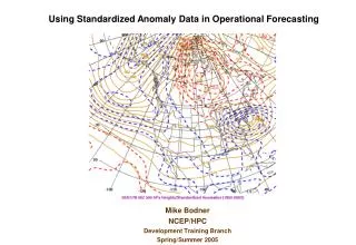
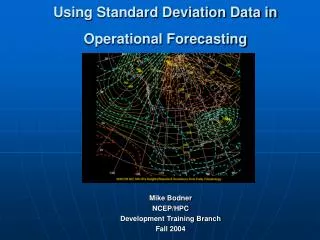
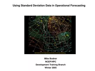
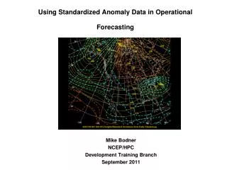
Using Standardized Anomaly Data in Operational Forecasting Mike Bodner NCEP/HPC Development Training Branch September 2011
Training Outline • Overview of standardized anomalies and statistical methods in forecasting • Methodology and computational information behind operational standard deviations • Application of standardized anomalies in forecasting • Case Study – Tennessee Flood – Spring 2010
Statistical or stochastic based tools already being used in forecasting… • MOS output • Ensembles • Bias corrected model data
Standardized anomalies are another tool to add to your forecaster tool chest… • Assess a meteorological feature based on 60 years of climatology • Can be applied to model forecast output • Fields can be compared to record breaking or extreme weather events from the past • Can use for model diagnostics and evaluation • Help discern pattern changes in medium range
How are standardized anomalies generated? • Daily averages and standard deviations (variances) are computed for several meteorological parameters using NCAR/NCEP Reanalysis data from 1948-2009 • A 15-day centered averaging is then applied to the daily data set • The 15-day filtered data is then subtracted from the model forecast, then divided by the standard deviation to get the standardized anomaly Note that the standardized or normalized data is “unit-less”. Therefore teleconnections can be derived between anomalies of different parameters.
Example using 500 hPa heights… Standard deviation or σ is computed by the following formula.. σ= square root of the average of Z2 - average Z2/ # years in data sample The number of standard deviations from the climatology or standardized anomaly is computed by subtracting the 60 year average height Z' from the model forecast or observed height Z, then dividing by the standard deviation σ Standardized Anomaly = (fcst height - average height) ÷ σ
Things to be mindful of when looking at standardized anomalies in forecasting… • Be aware of the standard deviation or variance pattern for your forecast data • Climatological variances are not as large over the southern latitudes, particularly during the warm season
An example of the computed standard deviations for 500 hPa heights forJuly 4. Notice how the variance increases proportionally with latitude. Also note how the largest standard deviations occur over the North Pacific and North Atlantic.
Let’s apply the SD data from the July 4 image in the previous slide… • At Atlanta, GA. The average 500 hPa height for July 4 is588 dm, and the standard deviation for 500 hPa height over Atlanta is3dm • A forecast value of 3 standard deviationsfrom normal or -3 would suggest a forecast height of 579 dm which is 9 dm below climatology • At Seattle, WA. The average 500 hPa height for July 4 is about 570 dm, and the standard deviation for 500 hPa height over Seattle is 9 dm • A forecast value of 3 standard deviationsfrom normal or -3 would suggest a forecast height of 543 dmor 27 dm below climatology.
Central U.S. Heat Wave 1980 Sample Application A prolonged heat wave gripped the central U.S. during the summer of 1980. The pattern featured a closed anti-cyclonic circulation at 500 hPa over the south central U.S. and 850 hPa temperatures 2-2.5 standard deviations above climatology. The charts displayed on the left are for July 14, 1980.
Record Cold Northeast U.S 19-21 January 1994 Temperatures remained below zero for over 50 hours in Pittsburgh and many other sections of Pennsylvania, Ohio New York and New England during 19-21 January 1994. 500 hPa height fields for 19 January 1994 show a deep trough over eastern North America, but the significant departure from climatology as depicted by the standard deviation fields illustrated the extent of the low level cold air.
850 hPa Moisture FluxHeavy Rain Event over CAOctober 2009 GFS 000HR forecast GFS 120HR Forecast +6.0 Sigma
Based on normal Gaussian distribution, the number of standard deviations (σ) are depicted along with the probability of occurrence with respect to climatology.
A standard PDF curve based on Gaussian distribution. The values plotted on the standard "bell curve" depict percent probability of a standard deviation being above or below the climatological mean (essentially these values are half of the probabilities sited in the above chart).
Disclaimer However, meteorological fields are not Gaussian distributed…therefore • Standardized anomaly data can NOT be used to determine the probability of the occurrence of an event • Data can NOT be used to estimate a 100 year or 500 year magnitude event Disclaimer
Estimating a PDF for a specific variable Since meteorological data does not typical fall in line with a Gaussian distribution, the ideal frame of reference for the standardized anomalies is a PDF for a given meteorological parameter on the respective model or reanalysis grid. Therefore we consider estimating a climatological probability using the Chebyshev Inequality. This is a probability theorem which states that in any data sample or probability distribution, nearly all the values are close to the mean values and provides a quantitative description of “nearly all” and “close to” Where σ = standard deviationk = standardized anomalyμ = meanX = random variable (height, temperature or other meteorological parameter) Therefore, no more than 1/k2 of the values are more than k standard deviations (where k is the value of the standardized anomaly) away from μ (the mean).
Let’s look at an example • If the GFS suggests a 120 hour forecast of 500 hPa Heights at -6.0 standard deviations below climatology, we can compute a climatological probability by taking the inverse reciprocal of the normalized anomaly value • Squaring this value • Multiplying the squared value by 1/2 (to account for both sides of the median) • Convert result to a percent • Therefore >> 1/62 = 1/36, 1/36 * ½ = 1/72, which = 0.0138 or 1.4% In other words, the probability that the 500 hPa heightswill differ from the climatological mean by more than 6 standard deviations is <= to 1.4%.Likewise the probability that the 500 hPa height will lie within 6 standard deviations of the mean is >= 98.6%
500 hPa heightforecast with standardized anomalies and climatological probabilities • Please be mindful that we are using model forecast data, and the various problems and biases of each model • This method accounts for climatological variance and provides a more reasonable climatological probability than extracting sigma values from a Bell Curve.
Sample of Precipitable Water, standardized anomalies, climatological probabilities
Total Precipitable Water 1200 UTC May 1, 2010 Tennessee FloodsMay 1-3, 2010 1200 UTC May 2, 2010 Rainfall Observations 24hrs ending 1200 UTC May 2 24hrs ending 1200 UTC May 3
500 hPa Geopotential HeightNormalized Anomalies(GFS Analysis) • Deep western U.S. trough • Anomalous Ridge along eastern seaboard • Favorable pattern for deep tropical moisture infusion into the Tennessee Valley region.
Precipitable Water Normalized Anomalies(GFS Analysis) • Deep western U.S. trough • Anomalous Ridge along eastern seaboard • Favorable pattern for deep tropical moisture pooling into the Tennessee Valley region.
- 3 standard dev (sigma) DRYMOIST ================================ subtropical jet - 5 standard dev (sigma) GFS 500mb Height Anomalies Initial VT 1200 UTC May 1, 2010 GOES Water Vapor 1215 UTC May 1, 2010 +2 sigma > 200% of normal ~ 175% of normal + 4 sigma GFS Precip Water Anomalies Initial VT 12 UTC May 1, 2010 Blended TPW Percent of Normal 1215 UTC May 1, 2010
850 hPa Moisture Flux (v * q)Normalized Anomalies(GFS Analysis) • Deep western U.S. trough • Anomalous Ridge along eastern seaboard • Favorable pattern for deep tropical moisture infusion into the Tennessee Valley region.
850 hPa V-Flux (meridional wind * q)Normalized Anomalies(GFS Analysis) • Depiction of tropical moisture originating in the deep tropics during high amplitude flow regime • Favorable assessment of “q” due to lower magnitudes of v-wind • Possible diagnostic for PRE events during the warm season
Midwest floods of 1993 and 2008 Normalized anomalies applied over a two week period
To sum up, when using standardized anomalies in the operational environment, always be mindful that… • It’s a statistical tool and not to be used to find an analogue from a “similar” past event, or assign a historical ranking to an event • Standardized anomalies are not a substitute for sound meteorological analysis, diagnosis and an informed forecast process • The tool is not to be used to assign a probability of occurrence for a specific weather event • Extreme SA values can be an indicator that a particular model solution may be going astray. • Although 850 hPa temperatures are below ground level in the west, the SAs correlate well with record events.
References Bodner, M.J., N.W. Junker, R.H. Grumm, R.S. Schumacher, 2011: Comparison of the 2008 Midwest floods to the historic 1993 floods: Atmospheric Circulation and Processes. Paper Accepted by National Weather Digest, February 2011. Kalnay, E., and Coauthers , 1996: The NCEP/NCAR 40-year Reanalysis Project. Bull. Amer. Meteor. Soc., 77, 437-471. Wilks, Daniel S., Statistical Methods in the Atmospheric Sciences, 2nd Edition, 2006.
Resources To view standardized anomaly data in real time, go to http://www.hpc.noaa.gov/training/SDs http://eyewall.met.psu.edu/ensembles To compute and display standardized anomaly data for specific a specific date(s) over your RFC/CWA, the web site below is an excellent reference. http://www.hpc.ncep.noaa.gov/ncepreanal Additional significant cases, including several on a more national scale can be found at the reference and training web site for using standard deviations. The web address is http://www.hpc.noaa.gov/training/ If you have questions or comments, please email mike.bodner@noaa.gov