Statistical Inference

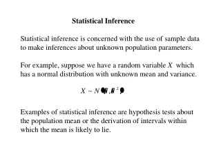
1. Statistical Inference Confidence intervals are one of the two most common types of statistical inference. Use a confidence interval when your goal is to estimate a population parameter. The second common type of inference, called tests of significance, has a different goal: to assess the evidence provided by data about some claim concerning a population. A test of significance is a formal procedure for comparing observed data with a claim (also called a hypothesis) whose truth we want to assess. • The claim is a statement about a parameter, like the population proportion p or the population mean µ. • We express the results of a significance test in terms of a probability that measures how well the data and the claim agree.

2. The Reasoning of Tests of Significance Suppose a basketball player claimed to be an 80% free-throw shooter. To test this claim, we have him attempt 50 free-throws. He makes 32 of them. His sample proportion of made shots is 32/50 = 0.64. What can we conclude about the claim based on these sample data? We can use software to simulate 400 sets of 50 shots assuming that the player is really an 80% shooter. You can say how strong the evidence against the player’s claim is by giving the probability that he would make as few as 32 out of 50 free throws if he really makes 80% in the long run. The observed statistic is so unlikely if the actual parameter value is p = 0.80 that it gives convincing evidence that the player’s claim is not true.

3. Stating Hypotheses A significance test starts with a careful statement of the claims we want to compare. The claim tested by a statistical test is called the null hypothesis (H0). The test is designed to assess the strength of the evidence against the null hypothesis. Often the null hypothesis is a statement of “no effect” or “no difference in the true means.” The claim about the population that we are trying to find evidence for is the alternative hypothesis (Ha). The alternative is one-sidedif it states that a parameter is larger or smaller than the null hypothesis value. It is two-sidedif it states that the parameter is differentfrom the null value (it could be either smaller or larger). In the free-throw shooter example, our hypotheses are: H0: p = 0.80 Ha: p < 0.80 where p is the true long-run proportion of made free throws.

4. Significance Test for a Proportion The z statistic has approximately the standard Normal distribution when H0is true. P-values therefore come from the standard Normal distribution. Here is a summary of the details for a z test for a proportion. z Test for a Proportion Choose an SRS of size n from a large population that contains an unknown proportion p of successes. To test the hypothesis H0: p = p0, compute the z statistic: Find the P-value by calculating the probability of getting a z statistic this large or larger in the direction specified by the alternative hypothesis Ha: Use this test only when the expected numbers of successes and failures are both at least 10.

6. Defining & Interpreting a P-value • Could random variation alone account for the difference between the null hypothesis and observations from a random sample? Compute the so-called P-value – the probability, assuming Ho true, that the test statistic takes on the observed value or a more “extreme” value (i.e., in the direction of the alternative hypothesis) • A small P-value implies that random variation due to the sampling process alone is not likely to account for the observed difference. • With a small p-value we reject H0. The true property of the population is significantly different from what was stated in H0. Thus, small P-values are strong evidence AGAINST H0. But how small is small…?

7. P = 0.2758 P = 0.0735 Significant P-value??? P = 0.1711 P = 0.05 P = 0.0892 P = 0.01 When the shaded area becomes very small, the probability of drawing such a sample at random gets very slim. Oftentimes, a P-value of 0.05 or less is considered significant: The phenomenon observed is unlikely to be entirely due to chance event from the random sampling.

8. Tests of statistical significance quantify the chance of obtaining a particular random sample result assuming the null hypothesis is true. This quantity is called the P-value. This is a way of assessing the “believability” of the null hypothesis, given the evidence provided by a random sample. The significance level, α, is the largest P-value tolerated for rejecting a true null hypothesis (how much evidence against H0 we require). This value is decided on arbitrarily before conducting the test. • If the P-value is equal to or less than α(P ≤ α), then we reject H0. • If the P-value is greater than α (P > α), then we fail to reject H0.

9. Example A potato-chip producer has just received a truckload of potatoes from its main supplier. If the producer determines that more than 8% of the potatoes in the shipment have blemishes, the truck will be sent away to get another load from the supplier. A supervisor selects a random sample of 500 potatoes from the truck. An inspection reveals that 47 of the potatoes have blemishes. Carry out a significance test at the α = 0.10 significance level. What should the producer conclude? We want to perform a test at the α = 0.10 significance level of H0: p = 0.08 Ha: p > 0.08 where p is the actual proportion of potatoes in this shipment with blemishes. • If conditions are met, we should do a one-sample z test for the population proportion p. • Random:The supervisor took a random sample of 500 potatoes from the shipment. • Normal:Assuming H0: p = 0.08 is true, the expected numbers of blemished and unblemished potatoes are np0= 500(0.08) = 40 and n(1 – p0) = 500(0.92) = 460, respectively. Because both of these values are at least 10, we should be safe doing Normal calculations.

10. Example The sample proportion of blemished potatoes is P-value The desired P-value is: P(z ≥ 1.15) = 1 – 0.8749 = 0.1251 Since our P-value, 0.1251, is greater than the chosen significance level of α = 0.10, we fail to reject H0. There is not sufficient evidence to conclude that the shipment contains more than 8% blemished potatoes. The producer will use this truckload of potatoes to make potato chips.

11. When the z score falls within the rejection region (shaded area on the tail-side), the p-value is smaller than α and you have shown statistical significance. z = -1.645 One-sided test, α = 5% Two-sided test, α = 1% Z

12. Rejection region for a two-tail test of p with α = 0.05 (5%) A two-sided test means that α is spread between both tails of the curve, thus:-A middle area C of 1 −α= 95%, and-An upper tail area of α/2 = 0.025. 0.025 0.025 Table C

13. Confidence intervals to test hypotheses Because a two-sided test is symmetrical, you can also use a confidence interval to test a two-sided hypothesis. If the hypothesized value of p is not inside the 100*(1-α) % confidence interval, then reject the null hypothesis at the α level, assuming a two-sided alternative. In a two-sided test, C = 1 – α. C confidence level α significance level α /2 α /2

14. Steps for Tests of Significance • Assumptions/Conditions • Specify variable, parameter, method of data collection, shape of population. • State hypotheses • Null hypothesis Ho and alternative hypothesis Ha often in terms of parameters • Calculate value of the test statistic • A measure of “difference” between hypothesized value and its estimate. • Determine the P-value • Probability, assuming Ho true, that the test statistic takes the observed value or a more “extreme” value. • State the decision and conclusion • Interpret P-value, make decision about Ho in context of the problem!

15. HW: Finish Reading Section 6.1 on Confidence Intervals and the new material on Significance Tests (See the box on page 357 for the Z-test). Watch the Stat Tutor Videos on Significance Testing on the Stats Portal. Work on Problems # 6.11- 6.14, 6.20, 6.22-6.24, 6.29-6.30, 6.32, 6.33, 6.35, 6.37