
Nonparametric Bayesian
E N D
Presentation Transcript
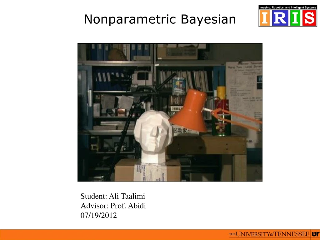
Nonparametric Bayesian Student: Ali Taalimi Advisor: Prof. Abidi 07/19/2012
Introduction • Machine learning is often split into three categories: • supervised learning: where a data set is split into inputs and outputs 2) reinforcement learning: where typically a reward is associated with achieving a set goal 3) unsupervised learning: where the objective is to understand the structure of a dataset.
Our Approach • One approach is unsupervised learning • How? • represent the data, Y, in some lower dimensional embedded space, X. • In a probabilistic model the variables associated with such a space are often known as latent variables. • our focus will be on methods that represent the data in this latent (or embedded)probabilistic latent variable models.
Previous Works probabilistic latent variable models has roots in approaches such as: density networks Using MLP: A prior distribution is placed over the latent-space and the latent-space’s posterior distribution is approximated. Density networks made use of the MLP to perform the mapping from Y to X (MacKay, 1995). Using RBF network: using RBF instead of MLP with the aim of decreasing the training time for the model (Bishop 1996). generative topographic mapping (GTM): (Bishop 1998) GPLVM: based on GTM and density network proximity data for visualization or embedding Multidimensional Scaling and Kernel PCA it is not obvious how to project back from the latent-space to the data-space or how to handle missing data. Isomap, LLE, Spectral Clustering
Problem Description • Y is in D dimensional space. • X is in d dimensional space. • GOALS: • Y X (embedding) • ability to embed a new sample y(n+1) without having to first return to the original training data (out-of-sample problem) • X Y (mapping from embedding space to original space/ pre-image problem) • preservation of relative distances in the embedding space. • Missing data Recovery (matrix completion)
Different Algorithms 1) Apply SVD on Y, with the columns of X defined by the weights on the d principal components. • XY: rank-d expansion using the d principal vectors, and the Frobenius norm between the original Y 2) preservation of inter-element L2 distances: • Motivated by Johnson-Lindenstrauss Lemma • XY is underdetermined. Y can be obtained PERFECTLY, if Y is sparsely represented in some basis (compressive sensing) 3) Using manifold Learning (Isomap, LLE, diffusion map, KPCA) • Unable to extract X Y, directly.(solution: landmarks) • Probabilistic-PCA, PPCA + Gaussian process latent variable model • Multi Factor Analysis
The focus of the paper Using LLE, Isomap, KPCA has a drawback! these methods generally suffer from an inability to perform the inversion from the embedding space, YX Solution: learning the embedding Y X by one of these methods, and then retaining exemplar yi for local regions of the embedding space; Question: what about number of such landmarks and their distribution? this paper presents a method for addressing this question using mixture factor models. Previous related statistical approaches: PPCA and GPLVM Model application: high-dimensional dynamic data, specifically motion-capture video Goal of application: inferring interrelationships between different portions of the time-dependent data The dynamic motion model is learned in the embedding space
Application • De-noising: Given a noisy image, de-noised image is obtained by computing the pre-image • Interpolation in the feature space (synthesize missing frames): silhouettes of a walking person are taken as training shapes and learned. Given a sequence of test silhouettes, some of the intermediate ones are discarded. The rest are mapped to the learned space, where linear interpolation is carried out to get the approximate mapping for the discarded shapes. The pre-image of the mappings are then carried out.
Face embedding and synthesis Fig1 of Pre-image Problem in Manifold Learning and Dimensional Reduction Methods VIDEO LINKS five straight line cuts (A–E) are shown in latent space, projected down to 2D. The endpoints of each cut (with colored borders) are images from the training set, while the intermediate images are synthesized. Fig6 of Hierarchical Bayesian Embeddings for Analysis and Synthesis of High-Dimensional Dynamic Data
nonparametric Bayesian methods • Bayesian statistics frames any problem of data analysis as one of updating beliefs about the world given observations. • Our beliefs are represented by a probability distribution over possible models of the world, and probabilistic inference is the mechanism by which our beliefs are updated. • field dedicated to placing probabilities on spaces larger than can be described by a finite dimensional vector (infinite dimensional space) • Gaussian process (continuous functions) • Dirichlet process discrete distributions • Poisson Process • Latent Variable Models
Why probabilistic inference in Machine Learning? probabilities provide a language for representing uncertainty. In machine learning we don’t have a set of rules that the machine knows about to find out the answer. rather we should show the machine some examples and machine should extract some regularities from them. But, we only show limited noisy examples, so the machine cannot be sure about things. observed data provide evidence for and against explanations: probably I have two different hypothesis about how the world looks like. Gathered data, maybe help to quantify the hypothesis.
Notation for probabilities • The joint probability of x and y is p(x, y). • The marginal probability of x is • The conditional probability of x given y is: • Bayes Rule is given by:
Notation for probabilities • The joint probability of x and y is p(x, y). • The marginal probability of x is • The conditional probability of x given y is: • Bayes Rule is given by:
Why, in principle, does Bayesian Inference work? Marginal likelihood is averaged over the likelihood weighted by the prior. So, if we have prior distribution which allows us to have lots of things, then we have to account all those things (even things that might not appear in the dataset==blue curve) from Rasmussen (Gaussian Process for Machine Learning)
Classical testing Example: We want to do a statistical test as to whether a new drug is helpful in treating high blood pressure. In a clinical trial, we measure the difference in blood pressure before and after treatment, with the new drug and a placebo (randomized, double blind, etc). Question: does the data cause us to reject the null hypothesis, H0, that the drug is no more efficient than the placebo (null hypothesis) The classical p-value measures how probable are the observations, or something more extreme, given that the null hypothesis is true? Note: in the classical test, the observations are considered random, and the unknown parameter assumed to be fixed.
Bayesian testing Find the posterior distribution (thing that we are interested in) of ∆ = ∆drug − ∆placebo. It uses the likelihood and prior over ∆. Report the probability that the drug works better than placebo: p(∆ > 0). Note: in the Bayesian test, the observed data are considered deterministic (because we see that it is not random anymore), but the unknown parameter considered random (here is the prob over ∆). misinterpreted of p value: people often says that p-value shows that the prob of the null hypothesis small.
Some vocabulary Bayesian inference is subjective as it depends on prior information. Bayesian inference obeys the likelihood principle: conclusions depend only on the likelihood of the observations (and the explicit model assumptions). The result of Bayesian inference is the posterior distribution, which captures everything you know, and let you talk about how the world work. To make decisions, minimize the expected value of the loss function averaged over the posterior. Loss func tells how expensive is it to make a particular guess about the state of the outcome when sth else happens to be truth. Minimizing such a cost is sometimes called Maximum A Posteri (MAP) estimates. A better name would be penalized maximum likelihood (non-Bayesian procedure).
Bayesian inference summary • Assumptions are made explicit in the form of a prior • Predictions are made by averaging over the posterior, taking all possible interpretations of the data into account • Bayesian inference does not involve any maximization so there is no possibility of over-fitting. Instead, parameters are integrated out. • Bayesian inference is usually difficult, because it is difficult to do integrals.
What is a Gaussian Process? • A Gaussian process is a generalization of a multivariate Gaussian distribution to infinitely many variables. • Informally: infinitely long vector ≃ function. If we just mention function f(x) in every x, then we specify the function. So this is infinitely long because it is specified for every possible x. • Definition: a Gaussian process is a collection of random variables, any finite number of which have (consistent) Gaussian distributions. • A Gaussian distribution is fully specified by a mean vector, μ, and covariance matrix Σ: f = (f1,...,fn)T ∼ N(μ,Σ), indexes i = 1,...,n • A Gaussian process is fully specified by a mean function m(x) and covariance function k(x, x′): • f (x) ∼ GP(m(x), k(x, x ′), indexes:x
The marginalization property Thinking of a GP as a Gaussian distribution with an infinitely long mean vector and an infinite by infinite covariance matrix may seem impractical. . . . . . luckily we are saved by the marginalization property: For Gaussians: Why marginalization is useful? because marginalization gives Gaussian (above formula) even if y variable is infinitely long. In fact even if y is infinitely long, it can say sth about some finite random variable (x)
Random functions from a Gaussian Process in fact GP, is the distribution over functions. When we want to have Bayesian inference, we need to specify prior distribution, so if we need distribution over functions, we need to specify prior over distribution of functions. Example one dimensional Gaussian process: p(f(x)) ∼ GP(m(x)=0, k(x,x′)=exp(−(x−x′)2/2)). Although the function has infinitely many entry, we plot the what the value of f has at certain set of x coordinates. we choose x1,…,xn, and see the value of function with distribution of f at those xs using marginalization.
Maximum likelihood, parametric model Supervised parametric learning: • data: x (input), y(output) • model: y = fw(x) + ε • ε ~ N(0, σ) Gaussian likelihood (probability of data given the parameters): To do inference, I should do maximum likelihood: Make predictions, by plugging in the ML estimate :
Bayesian Inference, parametric model, cont. After we got posterior distribution, we need to make inference Making predictions using the marginalization (inside the integral is joint probability of p(y*, w): is likelihood function evaluated at the test input. is posterior which is Gaussian. in fact we are calculating the p(y*) given new input (x*) and whatever we know about the model (w) and having observation(x, y). This integral is multiplication of two Gaussian distribution.
Non-parametric Gaussian process The parameters in nonparametric model is function itself. Wherever we have w in parametric model, we just plug in the function. In our non-parametric model, the “parameters” is the function itself! Gaussian likelihood: We are interested in particular observation(y), and y only depends on what the function is doing at that value of x. It doesn’t depend on the value of function in other points. This means that instead of conditioning on all the function values I can simply conditions on the function values at that locations (x). f are unknown, we don’t know what the function is. but I can at least write down that it depends on those which we collect at x.
Non-parametric Gaussian process (Zero mean) Gaussian process prior: Leads to a Gaussian process posterior (prior*likelihood): posterior is also a Gaussian process. And a Gaussian predictive distribution:
Some interpretation posterior variance(V(x*)) = prior variance – positive term Recall our main result: The mean is linear in two ways (because it is sth multiply to y): So the mean prediction, is the linear function of observations(y). Or it can be seen as linear function of kernels. So the mean can be assumed as linear in observations or linear in features. The variance is the difference between two terms:
The marginal likelihood Log marginal likelihood (integral of prior times likelihood) which helps us to compare models: is the combination of a data fit term(because it is the only term that depends on the data, data(y) is observations of the function values) and complexity penalty. Learning corresponds to find a good Covariance function. Learning in Gaussian process models involves finding • the form of the covariance function, and • any unknown (hyper-) parameters θ (parameters of model of Cov func ) optimize the marginal likelihood with respect to θ:
Example: Fitting the length scale parameter Parameterized covariance function: Cov func tells us, what is the covariance between the f values as a function of input values. If x and x’ are close, the corresponding f values should have high covariance. example of making inference abut length scale: plotting posterior mean function for 20 points of different values of length scale.
Model Selection in Practise; Hyperparameters Question: How can we use parameters to actually generate functions that could be useful for inference? There are two types of task: form and parameters of the covariance function. here we have three parameters, v0, v1, v2. long length scale means when x and x’ move away from each other, they have to move quiet far apart for function to change.