Image Localization and Geo-registration

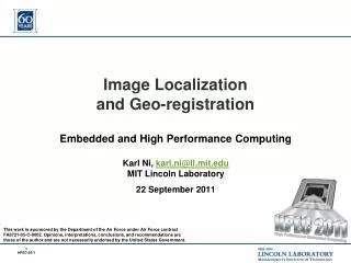
1. Image Localizationand Geo-registration Embedded and High Performance Computing Karl Ni, karl.ni@ll.mit.edu MIT Lincoln Laboratory 22 September 2011 This work is sponsored by the Department of the Air Force under Air Force contract FA8721-05-C-0002. Opinions, interpretations, conclusions, and recommendations are those of the author and are not necessarily endorsed by the United States Government.

2. Acknowledgements • Embedded and High Performance Computing (G102) • Karl Ni • Katherine Bouman • Scott Sawyer • Nadya Bliss • Active Optical Systems (G106) • Alexandru Vasile • Luke Skelly • Peter Cho • Cornell University • Noah Snavely

3. PED Vision DoD/IC Applications Target Capabilities Assessment Surveillance and Reconnaisance Multi-Platform & Handoff Online Mission Capabilities Social Network Analysis Tracking Multi-INTRepresentation Mission Planning Threat Assessment Geo-localization Geo-localization Navigation and Planning ExploitationProcessing Targeting and Recognition Detection of Hazardous Materials • Common representation enables a variety of exploitation products to work in a shared environment.

4. Geo-localization of Imagery and Video • Metadata • Graphs • Point Clouds • Distributions • Terrain • Etc. OFFLINESETUP Feature Extraction Matching & Association Ground Imagery, VideoAerial Imagery, Video FRAMEWORK Location Localization Algorithms World Model EXPLOITATION Multi-INTSources Processing

5. Challenges in Image Localization State of the Art Geo-localization DoD/IC Processing Capabilities SENSORS 2 City Blocks2, 0.12 miles2: Real-time Platform Capability = < 1 min (SIGMA Program, HPEC 2010) City-wide, 24 miles2: Parallel Computing Platform Estimated: 52 minutes USAScale (Land Only) Supercomputing Cluster Estimated: 22 days LLGRID • Large coverage of geo-spatial locations requires processing intelligently because coverage and precision scales with data.

6. Hierarchical Geo-localization • Coarse Classification • Medium Localization • Fine Geo-registration City! Forest! Cambridge BOS SF ORD NYC SF GPS (-42.32103, 72.1041, 29) +/- 100m • Reduce search space through successive localization • Confidence metric at each level

7. Outline • Introduction • Coarse Classification • . • Computational Complexity • Results • Medium Localization • Fine Geo-registration • Conclusions Medium Localization Feature Extraction Matching & Association Coarse Classification Fine Geo-registration

8. Coarse Feature: GIST Coarse Classification Feature Extraction Matching & Association Feature Extraction Matching & Association • The GIST Feature: • Naturalness • Openness • Roughness • Expansion • Ruggedness • Scene structure at various levels: • Subordinate level • Basic level • Superordinate level Spectral templates using windowed Fourier Transform Medium Localization Fine Geo-registration

9. Coarse Matching: GIST Mixtures • Comparing GIST Features: • Possible to do nearest neighbor approaches: computationally expensive • O(dNC) time, where N is exceedingly large • Using Gaussian Mixture Models • Model class distributions with a sum of several Gaussian • The number of Gaussians per class (P) is considerably smaller than N • Complexity proportional to O(dPC), where P is the number of Gaussians

10. Coarse Computational Loads Coarse Classification Feature Extraction Matching & Association Feature Extraction Matching & Association • GIST Feature computation • Dimensionality d = 960 vector comparisons • Each vector requires windowed FFT • Multiple resolutions and windowing • Parallel processing of different scales • Nearest neighbor O(dNC) • N = 487, C = 5, d = 960 • Comparison of 256^2 x N images x C Classes • Sparse feature GMM comparison O(dPC) • P = ~ 12/class, C = 5, d = 960 • Reduce computational complexity reduction on average 83.3%, up to 92.3%, depending on data • Two areas for parallelization: • Gaussian calculations are independent per prototype • Distribution value calculations are independent per class Medium Localization Fine Geo-registration

11. Coarse Coverage Capability and Results Coarse Classification • United States • 474M acres forest land • 349M acres crop land • 73M rural residential • 788M acres range and pasture land Medium Localization Fine Geo-registration • Training data set: 487 images spread across 5 different classes • Computation: 0.6 Seconds per image in MATLAB

12. Outline Coarse Classification • Introduction • Coarse Classification • Medium Localization • . • Computational Complexity • Results • Fine Geo-registration • Conclusions Feature Extraction Matching & Association Medium Localization Fine Geo-registration

13. Medium Features: Conceptual Coarse Classification Feature Extraction Matching & Association Feature Extraction Fine Geo-registration • FEATURES ARE: • Red bricks on multiple buildings • Small hedges, etc • Windows of a certain type • Types of buildings are there • FEATURES ARE: • More suburb-like • Larger roads • Drier vegetation • Shorter houses • FEATURES ARE: • Arches and white buildings • Domes and ancient architecture • Older/speckled materials (higher frequency image content) Medium Localization • Choice of features requires looking at multiple semantic concepts defined by entities and attributes inside of images

14. Medium Features: State of the Art (1/2) Coarse Classification • Face detection and recognition: mostly done • Generic object detector: not so much Fine Geo-registration Medium Localization

15. Medium Features: State of the Art (2/2) Coarse Classification • Let’s say you have 10 very good detectors (~%5 FA rate) • Still have a large image to classify at different scales/orientations and 10 x 0.05 FA rate for ~40% FA rate! • These classifiers don’t know anything about their surroundings! 7 Multiple Object Detector Results Person Detector without Context 5 2 1 Fine Geo-registration 6 4 3 People can’t be flying or walking on billboards 1. Chair, 2. Table, 3. Road, 4. Road, 5. Table, 6. Car, 7. Keyboard Medium Localization We use context in order inference about an image

16. Medium Features: Holistic Learned Features Coarse Classification • Feed noise + entire image into a sparse representation Feature Extraction Matching & Association Feature Extraction Automatic feature learning has been submitted to ICASSP 2012 Image Class N Image Class 2 Image Class 1 Fine Geo-registration Training images Training images Medium Localization Entire image Entire image Entire image Distribution N Distribution 2 Distribution 1 • Advantages: • Won’t need to segment every image • Will offer context information about surroundings and noise • Massively parallel per class

17. Medium Feature Matching: Distribution Analysis Coarse Classification Image Class N Feature Extraction Matching & Association Matching & Association Image Class 2 Image Class 1 Training images Training images Automatic feature learning has been submitted to ICASSP 2012 Entire image Entire image Entire image Fine Geo-registration Distribution N Distribution 2 Distribution 1 Image Class # Posterior Probability Calculations Medium Localization Input Test Image

18. Medium Computational Complexity Coarse Classification • Within Class Representation • 1400 images per dataset • Reduced resolution to 192 x 128 • Currently use 8x8 features • Potential features ~ 28 million per data set • Optimization  # features = 29 average filters (depending on thresholds) • Linear programming: single pass is O(dCN2), whereN = ~1400, C = 4 classes, d = 64 dimensions • Exploitation: • Comparisons are O(dCP), where P ~ 29 features • Less than a 30 seconds classification time (4 classes) • Coverage of cities: entire cities • Vienna • Dubrovnik • Lubbock • Portions of Cambridge (MIT-Kendall) Setup Fine Geo-registration Medium Localization World Model Exploitation

19. Results Coarse Classification Fine Geo-registration Medium Localization

20. Outline Coarse Classification • Introduction • Coarse Classification • Medium Localization • Fine Geo-registration • /. • Computational Complexity • Results • Conclusions Medium Localization Feature Extraction Matching & Association Fine Geo-registration

21. Scale/rotation invariant features are extracted and stored as vectors Fine Feature: SIFT Coarse Classification • SIFT at a glance: • Stands for: Scale Invariant Feature Transform • Scale Invariance: • Convolve Gaussian kernel at different scale factors • Rotation Invariance: • Bin gradient of local areas and build histogram Fine Geo-registration Number of Features per Image Comparison Average Number of Features Medium Localization Pixel Count X 106

22. Fine Feature Matching: Approx. Nearest Neighbor Coarse Classification Feature Extraction Matching & Association Matching & Association • Point cloud consists of averaged SIFT features at refined locations • Match to 2-D Features to 3-D Point Cloud • X is the matched feature position, d1, d2, are the feature distances, F is the representative feature Known 3-D Model Fine Geo-registration Medium Localization SIFT Features

23. Fine Computational Complexity • Each data set in the graph was run on 64 cores at a time using an MPI implementation • Each SIFT extraction is done on one core • Each image-image match is done on one core • 3D Reconstruction stage done in serial on one node Coarse Classification Setup Fine Geo-registration • Building 3D structure from known coordinates and matches is negligible in this framework • Majority of image geo-localization results can be processed in under or around a minute • Matching for larger data sets is more difficult Medium Localization World Model Exploitation

24. Fine Results Coarse Classification Fine Geo-registration PD Medium Localization Open Movie file Pfa

25. Overall Coverage and Complexity • Total dimensions • Coverage • Resolution • Complexity • Required data Exhaustive Search Required Data & Computation • Coarse localization: • Classification rate: best detection rate at 92.1% • Reduce search space by relative terrain classification • Classification confidence given by probabilistic GMM • GMM reduction in computation over state of the art (nearest neighbor) by N/C • Medium localization: • Demonstrated object classification per image: 79.2% • Localization passes in wholistic view of image to avoid supervision time • Massively parallel model building and training • Fine geo-registration • Demonstrated accuracy to within 4.7 meters • Feature matching and geo-registration in under a 1 minute per point cloud Coarse Processing Local Fine Coarse Coverage and Resolution

26. Conclusions • Placing overall framework onto a 3-D world representation model is advantageous in data exploitation • Geo-registration is feasibly done in a hierarchical manner, and determined via successive search-space reduction • There are various techniques that enable good registration in a timely fashion for classification and localization Feature Extraction Matching & Association

27. Questions?