Download
1 / 29
290 likes | 435 Vues
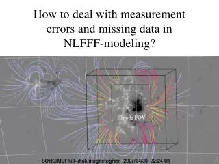
How to deal with measurement errors and missing data in NLFFF-modeling?. Hinode FOV. Conclusions from NLFFF-5. When presented with complete and consistent boundary conditions , NLFFF algorithms succeed in modeling test fields.

E N D
How to deal with measurement errors and missing data in NLFFF-modeling? Hinode FOV
Conclusions from NLFFF-5 • When presented with complete and consistent boundary conditions, NLFFF algorithms succeed in modeling test fields. • For a well-observed dataset (a Hinode/SOT-SP vector-magnetogram embedded in MDI data) the NLFFF algorithms did not yield consistent solutions. From this study we conclude that one should not rely on a model-field geometry or energy estimates unless they match coronal observations. • Successful application to real solar data likely requires at least: • large model volumes at high resolution that accommodate most of the connectivity within a region and to its surroundings; • accommodation of measurement uncertainties (in particular in the transverse field component) in the lower boundary condition; • 'preprocessing’ of the lower-boundary vector field that approximates the physics of the photosphere-to-chromosphere interface as it transforms the observed, forced, photospheric field to a realistic approximation of the high-chromospheric, near-force free field. • See: Schrijver et al. 2006 (SPh 235, 161), 2008 (ApJ 675, 1637), Metcalf et al. 2008 (SPh 247, 269), DeRosa et al. 2009 (ApJ 696, 1780).
Optimization Code force div B • Compute Potential field in simulation box. • Replace bottom boundary BT by data. • Minimize L numerically. • Data on boundaries remain unchanged. • L=0 corresponds to force-freeness and div B=0 • For inconsistent data L remains finite=> solution contains forces and/or finite div B
boundary data BT error matrix free pa- rameter New Optimization Code force div B • Compute Potential field in simulation box. • Minimize L numerically. • Bottom boundary BT becomes injected during iteration. Injection speed controlled by • Data on boundaries change during iteration. • L=0 corresponds to force-freeness, div B=0 andperfect agreement with boundary data. • For inconsistent data L remains finite, but with a small value of we still get a force and divergence free configuration.
Tests with Low & Lou Energy 93% Energy 99% BT missing for 85% of area 24% of flux Original ‘ideal’ magnetogram Potential 67% Energy 97% Energy 78% BT missing for 73% of area 14% of flux BT missing for 95% of area 49% of flux
original potential old, ideal new, ideal new, 85% missing old, 85% missing old, 95% missing new, 95% missing
Tests with Low and Lou:Evolution of force-freeness ‘L1’, div B ‘L2’ and deviation from vecmag ‘L3’ L1 L2 L3 New Code nu=0.01 Old Code Energy 99% Energy 99%
Old Code New Code nu=0.01 New Code nu=0.001 Tests with bad data. For 85% of the area and 24% of the flux we not had data for transversal field. BT =0, w=0 New Code: Configuration remains (almost) force-free and divergence-free during iteration. Energy 85% Energy 90% Energy 93%
Almost same results for old and new code for ideal data. Missing BT : div B, jxB=0, Energy better fulfilled with new code. Preprocessing improves div B, jxB=0 and Energy for both codes.
VC CS 1-NVE 1-MVE CWsin MAGEN RME <|f_i|> potl 1.0000 1.0000 1.0000 1.0000 0.8331 4.4494e+09 1.0000 1.0149e-10 Case1 potential Wieh 0.9850 0.9997 0.9502 0.9865 0.4671 4.6210e+09 1.0386 1.9560e-08 Wiegelmann masked1 Wieh 0.9898 0.9998 0.9628 0.9881 0.4698 4.6377e+09 1.0423 1.7438e-08 Wiegelmann masked2 Wieh 0.9871 0.9998 0.9603 0.9883 0.4952 4.6337e+09 1.0414 1.6673e-08 Wiegelmann masked3 Wieh 0.9849 0.9997 0.9484 0.9857 0.4699 4.6113e+09 1.0364 1.9688e-08 Wiegelmann masked4 Wie 0.9213 0.9749 0.7095 0.8102 0.4802 4.6644e+09 1.0483 2.0010e-07 Wiegelmann multigrid=3 Tha 0.9564 0.9908 0.8750 0.9653 0.5447 4.5163e+09 1.0151 4.2506e-07 Thalmann multigrid=1 Val 0.8521 0.8213 0.4033 0.3492 0.2898 4.0922e+09 0.9197 6.0762e-07 Valori1 Val 0.8795 0.9543 0.5790 0.7200 0.2911 4.7912e+09 1.0768 3.7688e-07 Valori2 McT 0.9011 0.9642 0.6497 0.8414 0.3641 5.0083e+09 1.1256 1.4087e-07 McTiernan Wh1- 0.9074 0.9440 0.5467 0.5890 0.1841 5.2910e+09 1.1892 1.2202e-08 Wheatland1- Wh1+ 0.9811 0.9641 0.7644 0.7172 0.2543 4.6228e+09 1.0390 5.1605e-08 Wheatland1+ Wh3 0.9845 0.9941 0.8308 0.8305 0.3405 4.5916e+09 1.0320 1.2828e-08 Wheatland3 Reg+ 0.9755 0.8934 0.6536 0.4038 0.4270 3.9063e+09 0.8779 5.0392e-08 Regnier+ Reg- 0.8872 0.8753 0.4855 0.3753 0.4076 4.7391e+09 1.0651 4.8508e-08 Regnier- Wh1b 0.8017 0.8823 0.2543 0.2835 0.3757 6.8137e+09 1.5314 3.5917e-08 Wheatland1b Can 0.8634 0.9001 0.4383 0.5023 0.1135 5.7637e+09 1.2954 1.3293e-08 Canou-XTRAPOL Am5 0.8558 0.9277 0.4016 0.2998 0.1049 5.9908e+09 1.3464 7.2153e-09 Amari-FEMQ-05b Am6 0.8700 0.9192 0.4215 0.2728 0.1325 5.7721e+09 1.2973 1.5169e-08 Amari-FEMQ-06 New Code is more divergence-free
A B C D potl 0.86 30.4 25.1 0.83 Case1 potential Wieh 0.86 30.5 25.3 0.83 Wiegelmann masked1 Wieh 0.86 30.5 25.2 0.83 Wiegelmann masked2 Wieh 0.86 30.5 25.2 0.83 Wiegelmann masked3 Wieh 0.86 30.5 25.3 0.83 Wiegelmann masked4 Wie 0.77 39.9 35.2 0.73 Wiegelmann multigrid=3 Tha 0.84 32.8 26.6 0.81 Thalmann multigrid=1 Val 0.52 58.6 57.4 0.52 Valori1 Val 0.80 36.9 32.2 0.77 Valori2 McT 0.71 44.5 40.8 0.68 McTiernan Wh1- 0.87 29.2 24.7 0.84 Wheatland1- Wh1+ 0.87 29.0 24.0 0.84 Wheatland1+ Wh3 0.87 29.8 24.6 0.83 Wheatland3 Reg+ 0.75 41.0 37.4 0.77 Regnier+ Reg- 0.76 40.7 37.9 0.77 Regnier- Wh1b 0.89 26.6 22.0 0.88 Wheatland1b Can 0.87 29.1 25.3 0.85 Canou-XTRAPOL Am5 0.86 31.0 27.4 0.84 Amari-FEMQ-05b Am6 0.86 30.9 27.4 0.85 Amari-FEMQ-06 column A = <cos(x)> column B = acos(<cos(x)>) column C = <x> column D = <Bcos(x)>/<B> New code Angle with STEREO-loops somewhat improved, but still unsatisfactory and comparable with potential field.
Trace Overlay New code
New code Fieldlines and iso-contours of |J|
New code Fieldlines and iso-surfaces of |J|
Application to MHD fromChip Manchester First NLFFF-test: z=50...209 (low beta regime) 300*300*160 box
First NLFFF-test: z=50...209 Bottom, |B| Front, y=0 Left, x=0 Back Right Top
Original MHD, z>=50 Potential, z>=50 Energy 78% NLFFF, old, multigrid, z>=50 NLFFF, new, multigrid, z>=50 Energy 96% Energy 96%
Full MHD Box 300x300x246 Bottom, |B| Front, y=0 Left, x=0 Magnetic Field Strength zero on parts of boundary Back Right Top
B=0 regions can be critical Magnetic Field Strength zero on parts of boundaryPotential problems: • We minimize the functional • Alternatively one could use Was somewhat slower for Low-Lou test done manyyears ago, but maybe worthwhile to explore againfor Chip’s MHD-case. Still to DO!
Potential , Full Box Original MHD, Full Box Energy 35% NLFFF new , Full Box NLFFF old , Full Box Energy 54-69% Energy 68%
Old and new codeprovided reasonable results for extrapolations from z=50 Chips MHD-case Force-free extrapolations from z=0 are unsatisfactory, but better than potential field.
How? Vecmag, z=0 z=0, Preprocessed, forces removed, but no good approximation for z=50 Vecmag, z=50
We tested preprocessing with Aad’s case For Aad’s case we well approximated z=2 from z=0 by preprocessing. Prepro- cessing Preprocessing does not help to get z=50 from z=0.
z=50, original from Chips MHD z=50, extrapolated with potential z=50, with NLFFF, multigrid 5 z=50, with MHS, multigrid 5 Extrapolations from z=0, almost full box 288*288*240
Non force-free computations • For real cases we do dot know the forces F. • Aim: Compute magnetic field, plasma pressure density self-consistently withMHS-code or extensions (plasma flow)and compare with original MHD cube. Computed in 3D from original MHD-cube
Summary • With consistent boundary data old and new code give basically the same result. • Error matrix in new code helps to get still reasonable results if BT missing or bad signal to noise ratio in part of area. • For inconsistent (missing data) input the new codeproduces better force and divergence-freeness. • Optimal free parameters have to be explored,nue=0.001 .... 0.01 and an assumed Error matrixw~| BT| or |B| look reasonable in first tests. • If BT missing in large parts of region/fluxthe result of new code is more potential.