aquatic ecosystem simulation modeling
Ecosystem Modeling and Hydrologic Modeling. Like hydrologic modeling, ecosystem modeling is primarily a matter of keeping track of a balance of flows.However, it is important to recognize some basic differences in practice.Ecosystem modeling is not as far along in having easily used

aquatic ecosystem simulation modeling
E N D
Presentation Transcript
1. Aquatic Ecosystem Simulation Modeling Don DeAngelisU.S. Geological Survey, Florida Integrated Science CentersMiami, Florida
Interdisciplinary Modeling for Aquatic EcosystemsLake Tahoe, July 17-22, 2005
3. Ecosystem Modeling and Hydrologic Modeling Some problems relate to the uniqueness of individual ecosystems:
Each ecosystem consists of its own suite of species populations, environmental conditions, spatial complexity, disturbance history, etc., that are unknown. In particular, the existence of thousands of poorly-understood species (with even less well known interactions) in an aquatic system always has the capacity to provide surprises.
Others relate to problems of complexity
Population interactions (predator-prey, competition, mutualism) are highly nonlinear (density dependent). We are not close to comprehending mathematically the complex dynamics that result from highly non-linear, multi-variable systems.
Together these create difficulty for predictive ecosystem modeling.
4. Aquatic Ecosystem Modeling My main points are:
Each ecosystem has to be considered carefully on its own and models crafted to fit that particular system.
Every �ecosystem model� will be limited to describing only certain aspects of the ecosystem.
Understanding output of dynamic model output (as opposed to the simpler description of �static� model flows) requires deep understanding of the behavior of nonlinear mathematics.
We can learn a great deal from ecosystem models (including some off the shelf models), but we cannot make many predictions with a high degree of confidence.
5. Ecosystem Modeling What I will do is: Discuss
What we mean by the structure of ecosystems.
How the static fluxes of energy can be described.
How material fluxes can be added to this.
How basic processes are modeled
How complex dynamic phenomena arise from nonlinearities in population (or functional group) interactions
Uncertainties
Resources
7. How do we describe the structure of flows of energy and matter in ecosystems?
This is done using methods of compartmental modeling, describing the changes in compartment sizes in terms of the inflows to and outflows.
Compartment sizes are the state variables of the system.
This leaves us with the difficult question of deciding what are the set of compartments.
8. Ecosystem Structure
10. But usually we need more disaggregated trophic structure, to include the food chain
11. A further conceptualization includes both �herbivore� and �detrital� food chains Another proposed representation would be to divide the ecosystem into separate herbivore and decomposer food chains, in view of the fact that these often are distinct, though they may share higher trophic levels.
14. Ecosystems Structure
Unfortunately, very few ecosystem models have been developed for ecosystems with this high a degree of resolution, and they each represent collective research done over decades.
15. Ecosystem Bioenergetics Describing the static energy flows
17. How do we determine the static flows of energy through the ecosystem?
Now we must also keep track of the gains and losses of each of these trophic levels. We can write an equation for the rate of change in each trophic level;
d(Biomassn)/dt = Instantaneous gross production (or assimilation of biomass consumed from lower trophic level)
- Losses (to respiration, natural mortality, predation)
= Gross Production - Respiration - Natural Mortality � Predation Mortality
= GP - R - NM - PM
'Biomass' and 'energy' or �carbon� are often used interchangeably, since biomass of organisms (e.g., in grams) can be converted to energy (e.g., in calories) by a simple conversion.
(Integration over time gives us biomass changes, BA, shown in preceding slide)
18. How do we determine the static flows of energy through the ecosystem? Raymond Lindeman (1941) applied this approach to aquatic ecosystems; Cedar Bog Lake and Lake Mendota.
Problem: It is really difficult to estimate most of the fluxes of the the individual functional groups.
The genius of Raymond Lindeman was to make useful simplifications.
First, he used a simple trophic level conceptualization of the aquatic ecosystem; I.e., aggregation of autotrophs, herbivores, primary and secondarycarnivores.
Second, he ignored natural mortality and assumed that all mortality was due to predation, also that the highest trophic level suffered no predation.
Third, he assumed a steady state (no net biomass accumulation in any trophic level through time) on a time scale from year to year.
20. Solving for energy flux through four trophic levels We can write equations:
dBiomass1/dt = Photosynthesis1 - R1 - PM1
dBiomass2/dt = a1 (PM1 - NA1 ) - R2 - PM2
dBiomass3/dt = a2 (PM2 - NA2) - R3 - PM3
dBiomass4/dt = a3 (PM3 - NA3) - R4
ai = assimilation by level i
21. Lindeman�s Solution A �steady state� occurs when the sizes of the various compartments do not change through time (at least when considered on a gross enough time scale); that it, there was no net accumulation; i.e., BA = 0. In that case one could assume that
dBiomass1/dt = dBiomass2/dt = dBiomass3/dt = dBiomass4/dt = 0
Thus, for the four trophic levels, he had a set of equations for energy balance
Trophic level 1 (Autotrophs)
Photosynthesis1 = R1 + PM1
Trophic level 2 (Herbivores)
PM1 - NA1 = R2 + PM2
Trophic level 3 (Carnivores)
PM2 - NA2 = R3 + PM3
Trophic level 4 (Second order carnivores)
PM3 - NA3 = R4
22. Lindeman�s Solution
Lindeman was able to obtain estimates of the fraction of consumed energy that is lost to egestion, NA, and the fraction of assimilated energy that is respired, R. That enabled him to determine the unknowns, PMi �s and Photosynthesis1
PM3 = NA3 + R4
PM2 = NA2 + R3 + PM3
PM1 = NA1 + R2 + PM2
Photosynthesis1 = R1 + PM1
23. How do we extend this static energy flow modeling to food webs? More detailed food web studies allow one to model ecosystems at a higher degree of resolution, applying the same type of energetic balance equations to food webs.
One needs information on:
Compartment sizes
Process rates (consumption, assimilation, respiration, etc.)
Diet composition
24. How do we extend this static energy flow modeling to food webs? Example:
Meyer and Poepperl developed a diagram of their food web. This includes 'Aufwuchs' or periphyton as the primary producer and base for herbivore, and also detritus as the base for the decomposer part of the web, although the herbivore and decomposer parts mesh at higher trophic levels.
It is impossible to try to account for every species population in an ecosystem, so these are grouped into 'guilds (often also called 'functional groups'), or 'groups of species having similar ecological resource requirements, foraging strategies, and predators'.
26. How do we extend this static energy flow modeling to food webs? Meyer and Poepperl were able to find empirical estimates of many of the process rates through studies on a particular stream over many years.
They also compiled data on 'who eats whom', or more precisely, how much of the diet of a consumer is made up of various prey.
These data do not directly tell us all of the flows. Meyer and Poepperl use the above input data, and then perform a mass-balance network analysis to find the 'matrix of flows' and other outputs, analogous to Lindeman�s approach, but much more sophisticated. This can also involve linear optimization techniques that construct the full set of flows that is completely balanced and matches the known flows as best as possible (e.g., Christensen and Pauly 1992, their ECOPATH, Diffendorfer, Richards, and DeAngelis, Ecological Modelling,1999?).
27. Ecosystem Material Fluxes Describing the static nutrient flows
31. Ecosystem Processes Describing the processes that drive flows
32. What are the ecosystem processes that drive fluxes of matter and energy?
Fluxes of energy and nutrients through ecosystems depend on processes of energy and material conversion.
The flows of energy and nutrients in ecosystems are governed by processes; primarily photosynthesis, respiration, consumption (herbivory and carnivory), and decomposition. (But there are actually many more, including spatial movement, that must often be taken into account.)
These are all complex and depend on densities of organisms, their physiology and behaviors, and environmental factors..
33. What are the ecosystem processes that drive fluxes of matter and energy?
Primary production (phytoplankton, periphyton, aquatic macrophytes)
The amount of photosynthesis is a given area is generally proportional to the biomass density, Biomass1. However, self-shading can occur, which requires a non-linear dependence.
Photosynthesis will be limited by either available light or nutrients, such as phosphorus or nitrogen, and the rate is proportional to a Michaelis-Menten factor, �N/(k + N), where N is nutrient concentration.
34. What are the ecosystem processes that drive fluxes of matter and energy?
We can write an expression for photosynthesis as
Photosynthesis = min[(�N/(k + N), f1(APAR, Biomass)]
*f2(Temperature)*Biomass1
where min[ . , . ] means that whichever factor, nutrient or available light (available photosynthetically active radiation, or APAR), is more limiting, that is smaller, will control the photosynthetic rate. The function f1 for the dependence of photosynthesis on APAR will depend on the physiology of the autotrophs, which may saturate at high light levels. Temperature also modulates the rate.
35. What are the ecosystem processes that drive fluxes of matter and energy? Heterotrophy and the functional response:
The rate of consumption of prey biomass by the consumer is usually modeled a linear function of consumer biomass (Biomassn) and a saturating function of prey biomass (Biomassn-1);
Consumption = a Biomassn-1 Biomassn /(1 + h Biomassn-1)
where a and h are constant parameters. The factor in the above equation multiplying Biomassn on the right hand side is called the functional response. So the loss of biomass from a prey compartment will increase linearly with consumer biomass, but not with prey biomass. High levels of prey biomass (1 < h Biomassn-1 ), will saturate the consumer�s ability to consume it.
36. What are the ecosystem processes that drive fluxes of matter and energy? Decomposition and nutrient recycling processes:
Decomposition may be highly complex because different materials decompose at different rates, depending on the type of biomass, and whether it is in the water column or sediment.
The array of processes that affect nutrient recycling can be highly complex, as in the case of nitrogen, which is first broken down through biomass decomposition into ammonia, hydrolyzes to ammonium ions, and may undergo nitrification to nitrate ions, and then denitrification to gaseous compounds that can escape into the atmosphere. This can be quantified in equations, but that is often very complex, depending on oxidation-reduction conditions, etc.
37. Question: What are the ecosystem processes that drive fluxes of matter and energy? Other processes:
Other processes that affect the above processes and may need to be modeling in certain situations include evapotranspiration, water movement and changes in depth, nutrient inputs and leaching, nutrient adsorption, sedimentation, removal of certain nutrients by complexing, organism migrations, and many more.
All processes can be modeled in various levels of detail.
38. Effects of Nonlinearities Emergence of complex phenomena in ecosystem models
39. What are the implications of nonlinearities for dynamics, structure, and flows?
Nonlinearities occur in ecosystem models because of the density dependencies in various processes.
The nonlinearities in the population interactions drastically affect the way ecosystems function.
This includes oscillatory behavior and chaos, as well as trophic cascades and mathematical catastrophes.
43. Mathematical catastrophes in ecosystems
Top-down effects can also lead to what are known as mathematical "catastrophes" in ecological systems. Such �catastrophes� are sudden changes that can occur in an ecosystem as the result of slow, gradual changes in an environmental parameter. These catastrophes involve shifts in which there is a change from one state of an ecosystem to another, usually with a change in dominance of the species community. These are of interest mathematically as well as ecologically, because they involve certain types of nonlinearities. (see especially, papers and book by Marten Scheffer.)
44. Consider a shallow lake that is relatively clear and has a lot of aquatic macrophytes on the bottom. Suppose there is a slow buildup of nutrients in the lake. For many years there is no discernible change in the lake�s biotic community. But suddenly, one summer, there is a big phytoplankton bloom. The bloom is there next year too, and soon the aquatic macrophytes die off.
To make matters worse, once the shallow lake has "tipped" from a clear, "macrophyte-dominated" lake to a turbid "algal-dominated" lake, it is not easy to change it back. Even if you are able to drastically reduce the nutrient input, the lake may not change back to its former clear self.
The above scenario has occurred very often in lakes. Theoretical ecologists have examined this phenomenon in terms of "mathematical catastrophe" theory, which is describes how a system may undergo major changes due to small changes in some environmental parameter.
45. The reason that such a dramatic change in the ecosystem can occur is that there are "self-reinforcing" processes occurring within a lake system (or any other ecosystem) that tend to maintain it in a stable state. But if you push the system too far, those self-reinforcing processes break down and turn against the original system.
46. Uncertainties Error propagation in complex ecosystem models
47. Yodzis�s Result Peter Yodzis (Ecology 1988) studied the propagation of uncertainty in large nonlinear food web models (> 12 or so species or functional groups).
He found that even if parameter values are known to within 15% or so, the propagation of uncertainty is such that, for a particular choice of parameters within the range of uncertainty, a perturbation in one functional group is equally likely to affect another given functional group positively or negatively.
.
48. Incompleteness of Ecosystem Models
Modeling means choosing what to include in a model system.
However, it is impossible to know a priori which components and processes in an ecosystem are likely to be important.
Hence, ecosystem models always are missing components and processes that may at some time be important in the modeled real system.
49. Lack of Analytic Understanding
Mathematical ecology has not supplied an understanding of the behavior of complex ecological systems; that is, nonlinear systems with more than two or three species.
Thus, analytic solutions cannot help us evaluate the output of model simulations.
50. Resources Packaged modeling platforms such as AQUATOX and EcoSim exist.
These should by all means be exercised as a part of experiencing the complexity of ecosystem behavior.
However, one should be aware of assumptions in these models, including ad hoc assumptions to maintain stability.
51. My view is that one should not trust the output of such packaged models unless one has a knowledge of the assumptions in the models and a deep understanding of nonlinear differential equation models.
For example, one should be able to understand the output of a model such as the following.
53. The equations take the form
54. Let�s assume that nutrient is completely recycled and there are no inputs or outputs of nutrient. The equations then can be written:
55. and let�s also assume
56. Evalutation of Model The model can be evaluated for sets of specific parameters; e.g.
ku = 0.05 khalf = 0.5 ka = 0.02
kh = 1.0 dplant = 0.02 dheter = 0.005
kdec,p = 0.01 kdec,h = 0.1 ? = 0.05
? = 0.02
If the total nutrient in the system, Ntotal, is allowed to vary, then the nutrient, plant biomass, and heterotroph biomass compartments behave as follows:
57. Equilibrium Values of Model Variables as Function of Total Nutrient
58. Analysis of Model It is also possible to examine the effects of other parameters. For example, suppose the total nutrient in the system, Ntotal, is held constant.
Let ku vary, representing changing rate of photosynthesis due to changes in solar radiation. Then the changes in the main variables are as in the following figure.
59. Equilibrium Values as Function of Solar RadiationTotal Nutrient in System Fixed.
60. Analysis of Model One can also study the temporal dynamics of the model for any given value of Ntotal by solving the set of differential equations plus constraint on nutrients.
Here, all other parameter values are fixed.
61. Ntotal = 2.0
62. Ntotal = 6.0
63. Ntotal = 9.0
64. The simple model here is about at the limits of what can easily be analyzed mathematically.
The model ignores the complexities of multiple limiting nutrients, of oxygen availability, carbon dioxide levels, etc., as it was developed for idealized ecosystems.
One should have an understanding of the behavior of such simple models before moving on to the more elaborate packaged aquatic ecosystem models.