Multi-layer Perceptrons and Solving XOR with Gradient Descent
Dive into the world of multi-layer perceptrons (MLPs) and their application in solving complex problems like XOR using techniques such as backpropagation with gradient descent. Explore challenges, solutions for local minima, training issues, and the essence of hidden layers in MLPs.

Multi-layer Perceptrons and Solving XOR with Gradient Descent
E N D
Presentation Transcript
Multi-layer perceptron Usman Roshan
Coordinate descent • Doesn’t require gradient • Can be applied to non-convex problems • Pseudocode: • for i = 0 to columns • while(prevobj – obj > 0.01) • prevobj = obj • wi += Δw • Recompute objective obj
Coordinate descent • Challenges with coordinate descent • Local minima with non-convex problems • How to escape local minima: • Random restarts • Simulated annealing • Iterated local search
Multilayer perceptrons • Many perceptrons with hidden layer • Can solve XOR and model non-linear functions • Leads to non-convex optimization problem solved by back propagation
Solving XOR with multi-layer perceptron z1 = s(x1 – x2 - .5) z2 = s(x2 – x1 - .5) y = s(z1 + z2 - .5)
Back propagation • Ilustration of back propagation • http://home.agh.edu.pl/~vlsi/AI/backp_t_en/backprop.html • Many local minima
Training issues for multilayer perceptrons • Convergence rate • Momentum • Adaptive learning • Overtraining • Early stopping
Another look at the perceptron • Let our datapoints xi be in a matrix form X = [x0,x1,…,xn-1] and let y = [y0,y1,…,yn-1] be the output labels. • Then the perceptron output can be viewed as wTX = yT where w is the perceptron. • And so the perceptron problem can be posed as
Multilayer perceptron • For a multilayer perceptron with one hidden layer we can think of the hidden layer as a new set of features obtained by a linear transformation of each feature. • Let our datapoints xi be in a matrix form X = [x0,x1,…,xn-1],y = [y0,y1,…,yn-1] be the output labels, and Z = [z0,z1,…,zn-1] be the new feature representation of our data. • In a single hidden layer perceptron we have perform k linear transformations W = [w1,w2,…,wk] of our data where each wi is a vector. • Thus the output of the first layer can be written as
Multilayer perceptrons • We convert the output of the hidden layer into a non-linear function. Otherwise we would only obtain another linear function (since a linear combination of linear functions is also linear) • The intermediate layer is then given a final linear transformation u to match the output labels y. In other words uTnonlinear(Z) = y’T. For example nonlinear(x)=sign(x) or nolinear(x)=sigmoid(x). • Thus the single layer objective can be written as • The back propagation algorithm solves this with gradient descent but other approaches can also be applied.