Multi Layer Perceptron
Multi Layer Perceptron. x 1. x 2. x n. Threshold Logic Unit (TLU). inputs. weights. w 1. output. activation. w 2. . y. q. a= i=1 n w i x i. w n. 1 if a q y = 0 if a < q. {. Activation Functions. threshold. linear. y. y. a. a.

Multi Layer Perceptron
E N D
Presentation Transcript
x1 x2 xn Threshold Logic Unit (TLU) inputs weights w1 output activation w2 y . . . q a=i=1n wi xi wn 1 if a q y= 0 if a< q {
Activation Functions threshold linear y y a a piece-wise linear sigmoid y y a a
Decision Surface of a TLU 1 1 Decision line w1 x1 + w2 x2 = q x2 w 1 0 0 0 x1 1 0 0
Geometric Interpretation The relation w•x=q defines the decision line x2 Decision line w y=1 w•x=q |xw|=q/|w| xw x1 x y=0
Geometric Interpretation • In n dimensions the relation w•x=q defines a n-1 dimensional hyper-plane, which is perpendicular to the weight vector w. • On one side of the hyper-plane (w•x>q) all patterns are classified by the TLU as “1”, while those that get classified as “0” lie on the other side of the hyper-plane. • If patterns can be not separated by a hyper-plane then they cannot be correctly classified with a TLU.
x1 x2 xn Threshold as Weight 1 if a 0 y= 0 if a<0 q=wn+1 xn+1=-1 w1 wn+1 w2 y . . . a= i=1n+1 wi xi wn {
Training ANNs • Training set S of examples {x,t} • x is an input vector and • t the desired target vector • Example: Logical And S = {(0,0),0}, {(0,1),0}, {(1,0),0}, {(1,1),1} • Iterative process • Present a training example x , compute network output y , compare output y with target t, adjust weights and thresholds • Learning rule • Specifies how to change the weights w and thresholds q of the network as a function of the inputs x, output y and target t.
Perceptron Learning Rule • w’=w + a (t-y) x Or in components • w’i = wi + Dwi = wi + a (t-y) xi (i=1..n+1) With wn+1 = q and xn+1=-1 • The parameter a is called the learning rate. It determines the magnitude of weight updates Dwi . • If the output is correct (t=y) the weights are not changed (Dwi =0). • If the output is incorrect (t y) the weights wi are changed such that the output of the TLU for the new weights w’i is closer/further to the input xi.
Perceptron Training Algorithm Repeat for each training vector pair (x,t) evaluate the output y when x is the input if yt then form a new weight vector w’ according to w’=w + a (t-y) x else do nothing end if end for Until y=t for all training vector pairs
Perceptron Convergence Theorem The algorithm converges to the correct classification • if the training data is linearly separable • and is sufficiently small • If two classes of vectors X1 and X2 are linearly separable, the application of the perceptron training algorithm will eventually result in a weight vector w0, such that w0 defines a TLU whose decision hyper-plane separates X1 and X2 (Rosenblatt 1962). • Solution w0 is not unique, since if w0 x =0 defines a hyper-plane, so does w’0= k w0.
x1 x2 xn Linear Unit inputs weights w1 output activation w2 y . . . y= a = i=1n wi xi a=i=1n wi xi wn
Gradient Descent Learning Rule • Consider linear unit without threshold and continuous output o (not just –1,1) • o=w0 + w1 x1 + … + wn xn • Train the wi’s such that they minimize the squared error • E[w1,…,wn] = ½ dD (td-od)2 where D is the set of training examples
(w1,w2) Gradient: E[w]=[E/w0,… E/wn] (w1+w1,w2 +w2) Gradient Descent D={<(1,1),1>,<(-1,-1),1>, <(1,-1),-1>,<(-1,1),-1>} w=- E[w] wi=- E/wi =/wi 1/2d(td-od)2 = /wi 1/2d(td-i wi xi)2 = d(td- od)(-xi)
Incremental Stochastic Gradient Descent • Batch mode : gradient descent w=w - ED[w] over the entire data D ED[w]=1/2d(td-od)2 • Incremental mode: gradient descent w=w - Ed[w] over individual training examples d Ed[w]=1/2 (td-od)2 Incremental Gradient Descent can approximate Batch Gradient Descent arbitrarily closely if is small enough
Perceptron vs. Gradient Descent Rule • perceptron rule w’i = wi + a (tp-yp) xip derived from manipulation of decision surface. • gradient descent rule w’i = wi + a (tp-yp) xip derived from minimization of error function E[w1,…,wn] = ½ p (tp-yp)2 by means of gradient descent. Where is the big difference?
Perceptron vs. Gradient Descent Rule Perceptron learning rule guaranteed to succeed if • Training examples are linearly separable • Sufficiently small learning rate Linear unit training rules uses gradient descent • Guaranteed to converge to hypothesis with minimum squared error • Given sufficiently small learning rate • Even when training data contains noise • Even when training data not separable by H
Presentation of Training Examples • Presenting all training examples once to the ANN is called an epoch. • In incremental stochastic gradient descent training examples can be presented in • Fixed order (1,2,3…,M) • Randomly permutated order (5,2,7,…,3) • Completely random (4,1,7,1,5,4,……)
x1 x2 xn Neuron with Sigmoid-Function inputs weights w1 output activation w2 y . . . a=i=1n wi xi wn y=s(a) =1/(1+e-a)
x1 x2 xn Sigmoid Unit x0=-1 w1 w0 a=i=0n wi xi y=(a)=1/(1+e-a) w2 y . . . (x) is the sigmoid function: 1/(1+e-x) wn d(x)/dx= (x) (1- (x)) • Derive gradient decent rules to train: • one sigmoid function • E/wi = -p(tp-y) y(1-y) xip • Multilayer networks of sigmoid units • backpropagation:
Gradient Descent Rule for Sigmoid Output Function s sigmoid Ep[w1,…,wn] = ½ (tp-yp)2 Ep/wi = /wi ½ (tp-yp)2 = /wi ½ (tp- s(Si wi xip))2 = (tp-yp) s‘(Si wi xip) (-xip) for y=s(a) = 1/(1+e-a) s’(a)= e-a/(1+e-a)2=s(a) (1-s(a)) a s’ a w’i= wi + wi = wi + a y(1-y)(tp-yp) xip
Gradient Descent Learning Rule wi = a yjp(1-yjp) (tjp-yjp) xip yj wji xi activation of pre-synaptic neuron learning rate error djof post-synaptic neuron derivative of activation function
Learning with hidden units • Networks without hidden units are very limited in the input-output mappings they can model. • More layers of linear units do not help. Its still linear. • Fixed output non-linearities are not enough • We need multiple layers of adaptive non-linear hidden units. This gives us a universal approximator. But how can we train such nets? • We need an efficient way of adapting all the weights, not just the last layer. This is hard. Learning the weights going into hidden units is equivalent to learning features. • Nobody is telling us directly what hidden units should do.
Learning by perturbing weights • Randomly perturb one weight and see if it improves performance. If so, save the change. • Very inefficient. We need to do multiple forward passes on a representative set of training data just to change one weight. • Towards the end of learning, large weight perturbations will nearly always make things worse. • We could randomly perturb all the weights in parallel and correlate the performance gain with the weight changes. • Not any better because we need lots of trials to “see” the effect of changing one weight through the noise created by all the others. output units hidden units input units Learning the hidden to output weights is easy. Learning the input to hidden weights is hard.
The idea behind backpropagation • We don’t know what the hidden units ought to do, but we can compute how fast the error changes as we change a hidden activity. • Instead of using desired activities to train the hidden units, use error derivatives w.r.t. hidden activities. • Each hidden activity can affect many output units and can therefore have many separate effects on the error. These effects must be combined. • We can compute error derivatives for all the hidden units efficiently. • Once we have the error derivatives for the hidden activities, its easy to get the error derivatives for the weights going into a hidden unit.
Multi-Layer Networks output layer hidden layer input layer
Training-Rule for Weights to the Output Layer Ep[wij] = ½ j (tjp-yjp)2 yj Ep/wji = /wji ½ Sj (tjp-yjp)2 = … = - yjp(1-ypj)(tpj-ypj) xip wji xi wji = a yjp(1-yjp) (tpj-yjp) xip = adjp xip with djp := yjp(1-yjp) (tpj-yjp)
Training-Rule for Weights to the Hidden Layer yj dj Credit assignment problem: No target values t for hidden layer units. wjk xk dk Error for hidden units? dk = Sj wjkdj yj (1-yj) wki wki = a xkp(1-xkp) dkp xip xi
Training-Rule for Weights to the Hidden Layer yj Ep[wki] = ½ j (tjp-yjp)2 dj wjk Ep/wki = /wki ½ Sj (tjp-yjp)2 =/wki ½Sj (tjp-s(Skwjk xkp))2 =/wki ½Sj (tjp-s(Skwjks(Siwki xip)))2 = -j (tjp-yjp) s’j(a) wjks’k(a) xip = -jdj wjks’k(a) xip = -jdj wjk xk (1-xk) xip xk dk wki xi wki = adk xip withdk = jdj wjkxk(1-xk)
Backpropagation Backward step: propagate errors from output to hidden layer yj dj wjk xk dk wki Forward step: Propagate activation from input to output layer xi
Backpropagation Algorithm • Initialize each wi to some small random value • Until the termination condition is met, Do • For each training example <(x1,…xn),t> Do • Input the instance (x1,…,xn) to the network and compute the network outputs yk • For each output unit k • k=yk(1-yk)(tk-yk) • For each hidden unit h • h=yh(1-yh) k wh,k k • For each network weight wi,j Do • wi,j=wi,j+wi,j where wi,j= j xi,j
Backpropagation • Gradient descent over entire network weight vector • Easily generalized to arbitrary directed graphs • Will find a local, not necessarily global error minimum -in practice often works well (can be invoked multiple times with different initial weights) • Often include weight momentum term wi,j(n)= j xi,j + wi,j (n-1) • Minimizes error training examples • Will it generalize well to unseen instances (over-fitting)? • Training can be slow typical 1000-10000 iterations (use Levenberg-Marquardt instead of gradient descent) • Using network after training is fast
Convergence of Backprop Gradient descent to some local minimum perhaps not global minimum • Add momentum term: wki(n) • wki(n) = adk(n) xi (n) + l Dwki(n-1) with l [0,1] • Stochastic gradient descent • Train multiple nets with different initial weights Nature of convergence • Initialize weights near zero • Therefore, initial networks near-linear • Increasingly non-linear functions possible as training progresses
Optimization Methods • There are other more efficient (faster convergence) optimization methods than gradient descent • Newton’s method uses a quadratic approximation (2nd order Taylor expansion) • F(x+Dx) = F(x) + F(x) Dx + Dx 2F(x) Dx + … • Conjugate gradients • Levenberg-Marquardt algorithm
NN: Universal Approximator? • Kolmogorov proved that any continuous function g(x) defined on the unit hypercube In can be represented as for properly chosen and .(A. N. Kolmogorov. On the representation of continuous functions of several variables by superposition of continuous functions of one variable and addition.Doklady Akademiia Nauk SSSR, 114(5):953-956, 1957)
Universal Approximation Property of ANN Boolean functions • Every boolean function can be represented by network with single hidden layer • But might require exponential (in number of inputs) hidden units Continuous functions • Every bounded continuous function can be approximated with arbitrarily small error, by network with one hidden layer [Cybenko 1989, Hornik 1989] • Any function can be approximated to arbitrary accuracy by a network with two hidden layers [Cybenko 1988]
Ways to use weight derivatives • How often to update • after each training case? • after a full sweep through the training data? • How much to update • Use a fixed learning rate? • Adapt the learning rate? • Add momentum? • Don’t use steepest descent?
Applications of neural networks • Alvinn (the neural network that learns to drive a van from camera inputs). • NETtalk: a network that learns to pronounce English text. • Recognizing hand-written zip codes. • Lots of applications in financial time series analysis.
NETtalk (Sejnowski & Rosenberg, 1987) • The task is to learn to pronounce English text from examples. • Training data is 1024 words from a side-by-side English/phoneme source. • Input: 7 consecutive characters from written text presented in a moving window that scans text. • Output: phoneme code giving the pronunciation of the letter at the center of the input window. • Network topology: 7x29 inputs (26 chars + punctuation marks), 80 hidden units and 26 output units (phoneme code). Sigmoid units in hidden and output layer.
NETtalk (contd.) • Training protocol: 95% accuracy on training set after 50 epochs of training by full gradient descent. 78% accuracy on a set-aside test set. • Comparison against Dectalk (a rule based expert system): Dectalk performs better; it represents a decade of analysis by linguists. NETtalk learns from examples alone and was constructed with little knowledge of the task.
Overfitting • The training data contains information about the regularities in the mapping from input to output. But it also contains noise • The target values may be unreliable. • There is sampling error. There will be accidental regularities just because of the particular training cases that were chosen. • When we fit the model, it cannot tell which regularities are real and which are caused by sampling error. • So it fits both kinds of regularity. • If the model is very flexible it can model the sampling error really well. This is a disaster.
Which model do you believe? The complicated model fits the data better. But it is not economical A model is convincing when it fits a lot of data surprisingly well. It is not surprising that a complicated model can fit a small amount of data. A simple example of overfitting
Generalization • The objective of learning is to achieve good generalization to new cases, otherwise just use a look-up table. • Generalization can be defined as a mathematical interpolation or regression over a set of training points: f(x) x
Generalization An Example: Computing Parity Can it learn from m examples to generalize to all 2^n possibilities? Parity bit value +1 +1 -1 >0 >1 >2 (n+1)^2 weights n bits of input 2^n possible examples
Generalization Network test of 10-bit parity (Denker et. al., 1987) 100% When number of training cases, m >> number of weights, then generalization occurs. Test Error 0 .25 .50 .75 1.0 Fraction of cases used during training
Generalization A Probabilistic Guarantee N = # hidden nodes m = # training cases W = # weights = error tolerance (< 1/8) Network will generalize with 95% confidence if: 1. Error on training set < 2. Based on PAC theory => provides a good rule of practice.
Generalization • The objective of learning is to achieve good generalization to new cases, otherwise just use a look-up table. • Generalization can be defined as a mathematical interpolation or regression over a set of training points: f(x) x
Generalization Over-Training • Is the equivalent of over-fitting a set of data points to a curve which is too complex • Occam’s Razor (1300s) : “plurality should not be assumed without necessity” • The simplest model which explains the majority of the data is usually the best
Generalization Preventing Over-training: • Use a separate test or tuning set of examples • Monitor error on the test set as network trains • Stop network training just prior to over-fit error occurring - early stopping or tuning • Number of effective weights is reduced • Most new systems have automated early stopping methods
Generalization Weight Decay: an automated method of effective weight control • Adjust the bp error function to penalize the growth of unnecessary weights: where: = weight -cost parameter is decayed by an amount proportional to its magnitude; those not reinforced => 0