
Comprehensive Guide to Classification in Data Mining by Dr. S. C. Shirwaikar" (89 characters)
E N D
Presentation Transcript
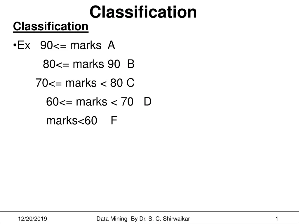
Classification • Classification • Ex 90<= marks A • 80<= marks 90 B • 70<= marks < 80 C • 60<= marks < 70 D • marks<60 F Data Mining -By Dr. S. C. Shirwaikar
Classification • Classification • predicts categorical class labels (discrete or nominal) • classifies data (constructs a model) based on the training set and the values (class labels) in a classifying attribute and uses it in classifying new data • Defn: Given a Database D={t1,t2,…tn} of tuples and a set C={C1,C2,…Cm}, the classification problem is to define a mapping f: D C where each ti is assigned to one class Cj. • Second Problem Overfitting Data Mining -By Dr. S. C. Shirwaikar
Classification • Three basic methods used to solve classification problems • Specifying boundaries • Using probability distributions p(ti/Cj) • Using posterior probabilities p(Cj/ti) Data Mining -By Dr. S. C. Shirwaikar
Typical applications • Credit approval-applicant as good or poor credit risk • Target marketing-profile of a good customer • Medical diagnosis- Develop a profile of stroke victims • Fraud detection -Determine a credit card purchase is fraudulent • Classification is a two-step process • Classifier is built from a data set- learning step • The training data set contains tuples having attributes one of which is a class label attribute Data Mining -By Dr. S. C. Shirwaikar
Example Training Data Set Attributes Class label • Supervised learning (classification) Data Mining -By Dr. S. C. Shirwaikar
Since class label is provided it is known as supervised learning Data Mining -By Dr. S. C. Shirwaikar
Model construction: • Describing a set of predetermined classes • Each tuple/sample is assumed to belong to a predefined class, as determined by the class label attribute • The set of tuples used for model construction is training set • The model is represented as classification rules, decision trees, or mathematical formulae • Model usage: • for classifying future or unknown objects • Estimate accuracy of the model The known label of test sample is compared with the classified result from the model • Accuracy rate is the percentage of test set samples that are correctly classified by the model • Test set is independent of training set, otherwise over-fitting will occur • If the accuracy is acceptable, use the model to classify data tuples whose class labels are not known Data Mining -By Dr. S. C. Shirwaikar
Swollen Glands No Yes Training Data Fever Diagnosis=Strep Throat Classifier (Model) No Yes Diagnosis=Allergy Diagnosis =Cold Classification Algorithms Data Mining -By Dr. S. C. Shirwaikar
Preparing data for classification • Data cleaning • Preprocess data in order to reduce noise and handle missing value • Ignore missing data • Assume a value for the missing data.This meas that the value of missing data is taken to be a specific value all of its own. Data Mining -By Dr. S. C. Shirwaikar
Relevance analysis (feature selection) • Remove the irrelevant or redundant attributes • Redundant attributes may be able to be detected by correlation analysis • Improves classification efficiency and scalability • Data transformation • Generalize and/or normalize data • -- Data Reduction Data Mining -By Dr. S. C. Shirwaikar
Choosing Classification Algorithms • Algorithm categorization • Distance based • Statistical • Decision Tree Based • Neural network • Rule based • Classification categorization • Specifying boundaries-divides input space into regions • Probabilistic- determine probability for each class and assign tuple to the class with highest probability Data Mining -By Dr. S. C. Shirwaikar
Measuring Performance • Performance of classification algorithm is by evaluating accuracy of the classification • Computational costs -Space and time requirements- • Scalability-efficient even for large databases • Robustness-ability to make correct classification in the presence of noisy data • Overfitting problem- the classification fits the training data exactly but may not be applicable to a broader population of data • Interpretability- insight provided by classifier Data Mining -By Dr. S. C. Shirwaikar
Statistical-based algorithms • Straight line regression analysis involves a response variable y and a single predictor variable x and models y is a linear function of x • y = w0 + w1 x • where w0 (y-intercept) and w1 (slope) are regression coefficients • These coefficients can be solved by the method of least squares which estimates the best fitting straight line • D be the training data set containing n data points (x1,y1),(x2,y2)…(xn,yn), regression coefficients can be estimated as • ∑ (xi- x) (yi –y) • w1 = ----------------------- w0 = y – w1 x • ∑ (xi- x)2 Data Mining -By Dr. S. C. Shirwaikar
100 80 60 40 20 x= 9.1 y =55.4 (3-9.1)(30-55.4)+……….. W1= ---------------------------------- = 3.5 W0 = 55.4-(3.5)(9.1)=23.6 (3-9.1)2 +(8-9.1)2……. y=23.6+3.5 x Using this equation we can predict salary given experience Data Mining -By Dr. S. C. Shirwaikar
Multiple Linear regression • It is an extension of Straight line regression analysis so as to involve more than one predictor variable • It allows response variable y to be modeled as a linear function of n predictor variables or attributes describing a tuple x as (x1,x2,…xn) • y = w0 + w1 x1 +w2 x2+w3x3+…..wnxn • The method of least squarescan be extended to solve for w0, w1 etc. the equations are much more complex and can be solved by using statistical software packages Data Mining -By Dr. S. C. Shirwaikar
The linear model gets affected by the presence of noise or outliers (extreme, exceptional values) Nonlinear regression • Some nonlinear models can be modeled by a polynomial function • A polynomial regression model can be transformed into linear regression model. For example, • y = w0 + w1 x + w2 x2 + w3 x3 • convertible to linear with new variables: x2 = x2, x3= x3 • y = w0 + w1 x + w2 x2 + w3 x3 • Some models are intractable nonlinear (e.g., sum of exponential terms) • possible to obtain least square estimates through extensive calculation on more complex formulae Data Mining -By Dr. S. C. Shirwaikar
Logistic regression • It uses a logistic curve. • The logistic curve gives a value between 0 and 1 so it can be interpreted as the probability of class membership. • The formula for a univariate logistic curve is • p= e (c0+c1x1) /1+ e (c0+c1x1) • log(p/1-p)=c0+c1x1 • Here p is the probability of being in the class e (1+x) /1+e (1+x) Data Mining -By Dr. S. C. Shirwaikar
Bayesian Classification: It is based on Bayes’ Theorem of conditional probability. It is a statistical classifier: performs probabilistic prediction, i.e., predicts class membership probabilities A simple Bayesian classifier, naïve Bayesian classifier, assumes that different attribute values are independent which simplifies computational process It has comparable performance with decision tree and selected neural network classifiers Data Mining -By Dr. S. C. Shirwaikar
Let X be a data tuple (“evidence”): described by values of its n attributes • Let H be a hypothesis that X belongs to class C • Classification is to determine P(H|X), the probability that the hypothesis holds given the observed data sample X • Probability that X belongs to class C having known the attribute description of X • Given that X is 31..40 and medium income , X will buy computer • P(H) (prior probability H ), the initial probability • E.g., X will buy computer, regardless of age, income, … Data Mining -By Dr. S. C. Shirwaikar
Let X be a data tuple (“evidence”): described by values of its n attributes • Let H be a hypothesis that X belongs to class C • Classification is to determine P(H|X), the probability that the hypothesis holds given the observed data sample X • Probability that X belongs to class C having known the attribute description of X • Given that X is 31..40 and medium income , X will buy computer • P(H) (prior probability H ), the initial probability • E.g., X will buy computer, regardless of age, income, … Data Mining -By Dr. S. C. Shirwaikar
P(H/X) (posteriori probability of H ), the probability of H when attributes of X are known • P(X): (prior probability of X) • It is probability that sample data is in observed range • Ex It is probability that person is in the range 31..40 and medium income- evidence • P(X/H) (posteriori probability of X) -likelihood • E.g.,Given that X will buy computer, the prob. that X is 31..40, medium income • Baye’s theorem relates all these probabilities • P(H/X)= P(X/H) P(H) • P(X) • Posteriori= Likelihood x priori / evidence Data Mining -By Dr. S. C. Shirwaikar
Let D be a training set of tuples and their associated class labels, and each tuple is represented by an n-D attribute vector X = (x1, x2, …, Xn) Suppose there are m classes C1, C2, …, Cm. Classification is to derive the maximum posteriori, i.e., the maximal P(Ci|X) This can be derived from Bayes’ theorem P(Ci/X)= P(X/Ci) P(Ci) P(X) Since P(X) is constant for all classes, only P(X/Ci)P(Ci) needs to be maximized Data Mining -By Dr. S. C. Shirwaikar
If class prior probabilities are not known, it can be assumed that all classes are equally likely P(C1)=P(C2) =………………..=P(Cn) Reduced to maximizing P(X/Ci) If data set has many attributes, it will be computationally expensive to compute P(X/Ci) To reduce computation, assumption of class conditional independence is made Attributes are conditionally independent P(X/Ci)= P(x1/Ci)xP(x2/Ci)x………………x P(xn/Ci) Data Mining -By Dr. S. C. Shirwaikar
P(xk/Ci) is the number of tuples of class Ci in training set D having the value xk, divided by number of tuples of class Ci in D Class: C1:buys_computer = ‘yes’ C2:buys_computer = ‘no’ Data sample X = (age <=30, Income = medium, Student = yes Credit_rating = Fair) Data Mining -By Dr. S. C. Shirwaikar
P(Ci): P(buys_computer = “yes”) = 9/14 = 0.643 • P(buys_computer = “no”) = 5/14= 0.357 • Compute P(X|Ci) for each class • P(age = “<=30” | buys_computer = “yes”) = 2/9 = 0.222 • P(age = “<= 30” | buys_computer = “no”) = 3/5 = 0.6 • P(income = “medium” | buys_computer = “yes”) = 4/9 = 0.444 • P(income = “medium” | buys_computer = “no”) = 2/5 = 0.4 • P(student = “yes” | buys_computer = “yes) = 6/9 = 0.667 • P(student = “yes” | buys_computer = “no”) = 1/5 = 0.2 • P(credit_rating = “fair” | buys_computer = “yes”) = 6/9 = 0.667 • P(credit_rating = “fair” | buys_computer = “no”) = 2/5 = 0.4 • X = (age <= 30 , income = medium, student = yes, credit_rating = fair) • P(X|Ci) : P(X|buys_computer = “yes”) = 0.222 x 0.444 x 0.667 x 0.667 • = 0.044 • P(X|buys_computer = “no”) = 0.6 x 0.4 x 0.2 x 0.4 = 0.019 • P(X|Ci)*P(Ci) : P(X|buys_computer = “yes”) * P(buys_computer = “yes”) • = 0.028 • P(X|buys_computer = “no”) * P(buys_computer = “no”) = 0.007 • Therefore, X belongs to class (“buys_computer = yes”) Data Mining -By Dr. S. C. Shirwaikar
Zero-probability problem • Naïve Bayesian prediction requires each conditional prob. to be non-zero. Otherwise, the predicted prob. will be zero irrespective of all other probabilities • Ex. Suppose a dataset with 1000 tuples, income=low (0), income= medium (990), and income = high (10), • Use Laplacian correction (or Laplacian estimator) • Adding 1 to each case • Prob(income = low) = 1/1003 • Prob(income = medium) = 991/1003 • Prob(income = high) = 11/1003 • The “corrected” prob. estimates are close to their “uncorrected” counterparts and the problem of zero probability is solved Data Mining -By Dr. S. C. Shirwaikar
Advantages • Easy to implement • Only one scan of training data is required • Good results obtained in most of the cases • Can easily handle missing values • Disadvantages • Assumption: class conditional independence, therefore loss of accuracy • Practically, dependencies exist among variables • E.g., hospitals: patients: Profile: age, family history, etc. • Symptoms: fever, cough etc., Disease: lung cancer, diabetes, etc. • Dependencies among these cannot be modeled by Naïve Bayesian Classifier • Bayesian Belief Networks Data Mining -By Dr. S. C. Shirwaikar
Distance-based algorithms Each tuple is assigned to class to which it is most similar Each class is represented as a tuple The representative for each class is the centre or centroid Each tuple ti is assigned to class Cj such that sim(ti,Cj) >sim(ti,Cl) for all Cl such that Cl≠Cj Each tuple must be compared to the center for a class and there are fixed number of classes. The complexity depends on the number of classes K Nearest Neighbors is a distance based algorithm i.e a lazy learning algorithm. Simply stores training data (or only does minor processing) and waits until it is given a test tuple Data Mining -By Dr. S. C. Shirwaikar
Distance-based algorithms • Similarity or distance measures may be used to identify the alikeness of different items in the database • The similarity between two tuples ti and tj sim(ti, tj) , in a database D is a mapping from DxD to the range [0,1] • Characteristics of a good similarity measure • sim(ti, ti)=1 for all ti • sim(ti, tj)=0 if ti and tj are not alike at all • sim(ti,tj) < sim(ti, tk) if ti is more like tk than it is like tj Data Mining -By Dr. S. C. Shirwaikar
Dice: sim(ti,tj) = ∑ tik tjk ∑ tik2 + ∑tjk2 Jaccard : sim(ti,tj) = ∑ tik tjk ∑ tik2 +∑tjk2 - ∑ tik tjk Cosine : sim(ti,tj) = ∑ tik tjk ∑ tik2 ∑tjk2 Overlap : sim(ti,tj) = ∑ tik tjk min (∑ tik2, ∑tjk2) Distance or dissimilarity measures are often used instead of similarity measures-usually distance measures Euclidean : dis(ti,tj) = ∑ (tih-tjh)2 Manhattan : dis(ti,tj) = ∑ | tih-tik| Data Mining -By Dr. S. C. Shirwaikar
The k-Nearest neighbor algorithm • K closet neighbors in the training set to the given tuple are to be determined • The nearest neighbor are defined in terms of Euclidean distance, dist(X1, X2) • The new item is then placed in the class that contains the most items from this set k of closest items • The value of k can be determined experimentally. Starting with k=1, a test set is used to estimate the error rate of the classifier. The k value that gives minimum error rate can be selected • k-NN for real-valued prediction for a given unknown tuple returns the mean values of the k nearest neighbors Data Mining -By Dr. S. C. Shirwaikar
The k-Nearest neighbor algorithm • Distance-weighted nearest neighbor algorithm gives greater weight to closer neighbors • Robust to noisy data by averaging k-nearest neighbors • The complexity is O(d), d is the size of training set, can be reduced to O(logd) by storing training set in search trees, can be O(1) by using parallelism Data Mining -By Dr. S. C. Shirwaikar
Swollen Glands No Yes Fever Diagnosis=StrepThroat No Yes Diagnosis=Allergy Diagnosis =Cold Decision Tree based algorithms A decision tree is a flowchart like tree structure , where each internal node denotes a test on an attribute, each branch represents an outcome of the test and each leaf node holds a class label A path is traced from the root to a leaf node, which holds the class prediction for that tuple Data Mining -By Dr. S. C. Shirwaikar
age? <=30 overcast >40 31..40 student? credit rating? customer excellent fair no yes customer Non-Customer Non-customer customer Data Mining -By Dr. S. C. Shirwaikar
Algorithm Generate_decision_tree(D, attribute_list) • Create a Node N • If tuples in D are in the same class C then return N as leaf node labeled with class C • If attribute list is empty then return N as a leaf node labeled with the majority class in D • Apply attribute selection method D to get the best splitting attribute and label the node accordingly • Split the node depending on attribute domain • For each split • Let Dj be the set of data tuples in D satisfying outcome j • If Dj is empty then attach a leaf labeled with majotrity class in D • Else give a recursive call to Generate _decsion tree for the new node Data Mining -By Dr. S. C. Shirwaikar
Decision_Tree induction: • Construct a DT using training data • For each ti € D,apply the DT to determine it’s class. • Advantages: • 1.Easy to use and efficient • 2.Rules can br generated that are easy to interpret and understand. • 3.They scale well for large databases because the tree size is independent of database size. Data Mining -By Dr. S. C. Shirwaikar
Input- • D //training data • Output:- • T //Decision Tree • DTBuild algorithm: • T= ø • Determine best splitting criterion: • T= Create root node and label with splitting attribute; • T= Add arc to root node for each split predicate and label; • for each arc do • D = Database created by applying splitting predicate to D; • If stopping point reached for this path,then • T’= Create leaf node and label with appropriate class; • else • T’=DTBuild(D); • T’= Add T’ to arc; Data Mining -By Dr. S. C. Shirwaikar
Disadvantages: 1.They do not easily handle continuous data 2. These attribute domain must be divided into categories to be handled. 3. Data Mining -By Dr. S. C. Shirwaikar
Issues faced by DT algorithms • Choosing splitting attributes -best splitting criterion is when all tuples in the partition belong to the same class(pure). Some attributes are better than other. • Choice of attribute should be such that it minimizes the expected number of tests needed to classify a given tuple and guarantees a simple tree structure • Ordering of splitting attributes – The order in which the attributes are chosen is important • The attributes are ranked based on some attribute selection measure. The best score attribute is chosen as splitting attribute • Splits- number of splits depends on the domain of the attribute • Tree structure- a balanced tree with the fewest levels is desirable Data Mining -By Dr. S. C. Shirwaikar
Stopping criteria – The creation of the tree stops when the training data is perfectly classified. Stopping earlier can prevent overfitting and generation of large trees • Training data –Training data set can give rise to overfitting problem • Pruning- Once a tree is constructed ,some modifications to the tree might not be specific enough to work properly with more general data. • ID3(Iterative Dichotomiser) • ID3 technique of building a decision tree is based on information theory and attempts to minimize excepted number of comparisons • Like in “Twenty question Game” ask questions that provide the most information Data Mining -By Dr. S. C. Shirwaikar
Entropy is used to measure the amount of uncertainity or surprise in a set of data When all data in a set belongs to the same class there is no uncertainity – entropy is zero The objective of decision tree classification is to iteratively partition the given data set into subsets where all elements in each final subset belong to the same class-pure partition Defn : Given a data set D and probabilities p1,p2,…pn where ∑ pi=1,pi is the probability that an arbitrary tuple in D belongs to Class Ci, entropy or expected information neededd to classify a tuple in D is defined as H(D)= ∑ pi (log(1/pi)) = - ∑ pi log(pi) Data Mining -By Dr. S. C. Shirwaikar
If selection of an attribute A does not result into pure partitions then additional information required in order to arrive at exact classification is measured as infoA(D) = ∑|Dj|/|D| x Info(Dj) The term |Dj|/|D| acts as the weight of the jth partition Information gained by branching on attribute A Gain(A)=Info(D)-InfoA(D) The difference between the original information requirement based on just the proportion of classes and the new requirement obtained after partitioning on A The smaller the expected information ,the greater is the purity of the partitions Select the attribute with the highest information gain Data Mining -By Dr. S. C. Shirwaikar
H(D) = Info(D) = -9/14 log(9/14) – 5/14 log (5/14) =0.940 If the tuples are classified according to attribute age The Expected information required for further classification after partitioning on Attribute age Info age(d) = 5/14 x( -2/5log(2/5)-3/5log(3/5)) + 4/14 x( -4/4log(4/4)-0/4log(0/4)) + 5/14 x( -3/5log(3/5)-2/5log(2/5)) = 0.694 bits Hence gain in information Gain(age) = Info(d) – Infoage(D) = 0.940-0.694=0.246 Similarly gains for other attributes can be calculated Gain(Income) =0.029 Gain(student)=0.151 and Gain(credit_rating)=0.048 Hence attribute age is chosen as the splitting attribute Data Mining -By Dr. S. C. Shirwaikar
C4.5 is a successor of ID3 It improves ID3 in the following ways Missing data- instead of ignoring missing data , the value is predicted based on what is known about the attributes of other records Continuous data- discretized by dividing data into ranges Pruning- - with subtree replacement , a subtree is replaced by a leaf node, if this replacement results in an error rate close to that of the original tree –bottom up -With Subtree raising, a subtree is replaced by its most used subtree. Subtree is raised to a higher location depending on increase in error rate Data Mining -By Dr. S. C. Shirwaikar
Rules - generates both decision tree and the rules set. . Some methods are used to simplify rules such as replacing rule by a simpler version Splitting – The ID3 approach favors attributes with many divisions and thus may lead to overfitting . An improvement can be made by taking into account the cardinality of each division. The GainRatio is used opposed to Gain GainRatio(D,S)= Gain(D,S) / H(|Di|/|D|) C 4.5 uses the largest Gainratio that ensures larger than average Information gain For the attribute Income H(|Di|/|D|) = -4/14log(4/14) -6/14log(6/14) – 4/14log(4/14) = 0.926 Gainratio= Gain(Income)/0.926=0.029/0.926=0.031 Data Mining -By Dr. S. C. Shirwaikar
CART (Classification and regression trees ) is a technique that generates a binary decision tree Entrpy is used as a measure to chose the best splitting attribute In ID3 one child is created for each subcategory while here only two children are created At each step , exhaustive search is used to decide the best split where best is defined by Φ(s/t) = 2PLPR∑ | P(Ci / tL) – P (Ci / tR )| Here L and R indicate left and right subtrees, PL and PR are the probabilities that the tuple will be on left or right side of the tree P(Ci/TL) denote the probability a tuple is in classs Ci and in the left subtree Data Mining -By Dr. S. C. Shirwaikar
Scalable DT technique SPRINT(Scalable Parallelizable Induction of decision tree It addresses scalability issue by adding parallelism It uses gini index to find the best split If a data set D contains examples from n classes, gini index, gini(D) is defined as gini(D)= 1 - ∑ pj2 where pj is the relative frequency of class j in D If a data set D is split on A into two subsets D1 and D2, the gini index gini(D) is defined as gini split (D) = n1/n ginii(D1)+ n2/n gini(D2) The attribute provides the smallest ginisplit(D) (or the largest reduction in impurity) is chosen to split the node (need to enumerate all the possible splitting points for each attribute) Data Mining -By Dr. S. C. Shirwaikar
Neural Networks is an information processing system in the form of a graph with many nodes as processing elements (Neurons) and arcs as interconnections between them. NN can be viewed as a directed graph with source (input), sink (output) and internal (hidden) nodes. The input nodes exist in the input layer, output nodes in the output layer and hidden nodes in one or more hidden layers During processing , functions at each node are applied to the input data to produce the output Data Mining -By Dr. S. C. Shirwaikar