Multidimensional Scaling Analysis of Water Vole Populations Using R
100 likes | 222 Vues
This analysis employs R to create a classical scaling solution for water vole populations, identifying the number of dimensions suitable for representation through the Trace and Magnitude criteria. It reveals that the original distances between populations can be adequately represented in two dimensions. The study visualizes the results using a plot with coordinates and highlights potential distortions through a Minimum Spanning Tree. Additionally, an example of non-metric scaling is provided, assessing voting behavior among Republicans, illustrating the variability in their voting patterns.

Multidimensional Scaling Analysis of Water Vole Populations Using R
E N D
Presentation Transcript
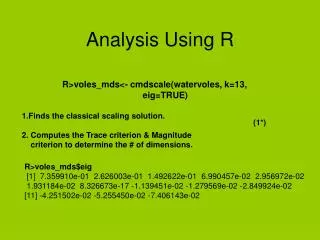
Analysis Using R 1.Finds the classical scaling solution. 2. Computes the Trace criterion & Magnitude criterion to determine the # of dimensions. (1*) R>voles_mds<- cmdscale(watervoles, k=13, eig=TRUE) R>voles_mds$eig [1] 7.359910e-01 2.626003e-01 1.492622e-01 6.990457e-02 2.956972e-02 1.931184e-02 8.326673e-17 -1.139451e-02 -1.279569e-02 -2.849924e-02 [11] -4.251502e-02 -5.255450e-02 -7.406143e-02
We have 13 eigenvalues, some positive & some negative. R>sum(abs(voles_mds$eig[1:2]))/ sum (abs(voles_mds$eig)) [1] 0.6708889 This code satisfies Magnitude Criterion. (2*) R>sum((voles_mds$eig[1:2])^2/ sum((voles_mds$eig)^2) [1] 0.9391378 Which is the criteria suggested by Mardia et al.; the above code is exactly: k n ∑│λ│ / ∑ │λ│ i=1 i=1 0.6708889 & .9391378 are large enough to suggest that the original distances Between water vole populations can be represented adequately in two dimensions. (3*)
R>x<- voles_mds$points[, 1] 1: Coordinate 1 R>y<-voles_mds$points[, 2] 2: Coordinate 2 R>plot(x,y,xlab= "Coordinate 1", ylab= "Coordinate 2", xlim= range(x) * 1.2, type= "n") R>text(x,y, labels= colnames(watervoles)) 6 British populations are close to populations living in the Alps, Yugoslavia, Germany, Norway, & Pyrenees I. (Arvicola terrestris) These British populations are distant from the populations in Pyrenees II, North Spain and South Spain. (Arvicola sapidus) (4*)
Minimum Spanning Tree (MDS solution) highlight possible distortions. (5,6*) Links of a minimum spanning tree of the proximity matrix may be plotted onto the two-dimensional scaling representation to identify distortions (if any) produced by scaling solutions. These distortions look like nearby points on the plot that are not linked by an edge of a tree. (7*) R>library("ape") R>st<- mst(watervoles) R>plot(x,y,xlab= "Coordinate 1", ylab= "Coordinate 2", xlim= range (x) * 1.2, type= "n") R>for (i in 1:nrow(watervoles)) { + w1<- which(st[i, ] == 1) + segments(x[i], y[i], x[w1], y[w1]) } R>text(x, y, labels= colnames(watervoles))
The apparent closeness of the populations, Germany & Norway, by the points suggested here in this MDS solution, does not reflect accurately their calculated dissimilarity. (8*)
Non-Metric Scaling Example: Analyzing Voting Behavior among Republicans. R Function isoMDS from package “MASS” R>library("MASS") R>data("voting", package= "HSAUR") R>voting_mds<- isoMDS(voting)
Two-Dimensional Solution: R>x<- voting_mds$points[, 1] R>y<- voting_mds$points[, 2] R>plot(x,y, xlab="Coordinate 1", ylab= "Coordinate 2", + xlim= range(voting_mds$points[, 1]) *1.2, + type= "n" ) R>text(x,y, labels= colnames(voting)) R>voting_sh<- Shepard(voting[ lower.tri(voting)], + voting_mds$points Figure suggests that there is more variation in voting behavior among Republicans. (*9)
R>library("MASS") R>voting_sh<- Shepard(voting[lower.tri(voting)], + voting_mds$points) R>plot(voting_sh, pc= ".", xlab= "Dissimilarity", + ylab= "Distance", xlim= range(voting_sh$x), + ylim= range(voting_sh$x)) R>lines(voting_sh$x, voting_sh$yf, type= "S") Quality of a multidimensional scaling can be assessed informally by plotting the original dissimilarities & the distances obtained from a multidimensional scaling in a scatterplot. Ideally, all the lines should fall on the bisecting line.