Download

1 / 66
660 likes | 763 Vues
Explore the transition in evolutionary studies from anatomical features to DNA analysis to derive relationships between species. Understand the Out of Africa Hypothesis and the Origin of Humans, contrasting it with the Multiregional Hypothesis, utilizing evolutionary trees constructed from mtDNA and microsatellites. Learn about different methods used to build phylogenetic trees and establish distances in evolutionary paths. Witness the complexity of reconstructing unknown tree topologies from DNA sequences and explore tree reconstruction principles for varying levels of tree leaves.

E N D
CSCI2950-C Lecture 7Molecular Evolution and Phylogeny http://cs.brown.edu/courses/csci2950-c/
Early Evolutionary Studies • Anatomical features were the dominant criteria used to derive evolutionary relationships between species since Darwin till early 1960s • The evolutionary relationships derived from these relatively subjective observations were often inconclusive. Some of them were later proved incorrect
Evolutionary Trees from DNA analysis • For roughly 100 years scientists were unable to figure out which family the giant panda belongs to • Giant pandas look like bears but have features that are unusual for bears and typical for raccoons, e.g., they do not hibernate • In 1985, Steven O’Brien and colleagues solved the giant panda classification problem using DNA sequences and algorithms
1 2 3 4 5 http://www.becominghuman.org Out of Africa Hypothesis • DNA-based reconstruction of the human evolutionary tree led to the Out of Africa Hypothesis thatclaims our most ancient ancestor lived in Africa roughly 200,000 years ago
Human Evolutionary Tree http://www.mun.ca/biology/scarr/Out_of_Africa2.htm
The Origin of Humans: ”Out of Africa” vs Multiregional Hypothesis Out of Africa: • Humans evolved in Africa ~150,000 years ago • Humans migrated out of Africa, replacing other humanoids around the globe • Multiregional: • Humans evolved in the last two million years as a single species. Independent appearance of modern traits in different areas • Humans migrated out of Africa mixing with other humanoids on the way
Evolutionary Tree of Humans (mtDNA) • African population is the most diverse • (sub-populations had more time to diverge) • Evolutionary tree separates one group of Africans from a group containing all five populations. • Tree rooted on branch between groups of greatest difference. Vigilant, Stoneking, Harpending, Hawkes, and Wilson (1991)
Evolutionary Tree of Humans: (microsatellites) • Neighbor joining tree for 14 human populations genotyped with 30 microsatellite loci.
Outline • Constructing Phylogenetic Trees • Distance-based Methods • Additive distances • 4 Point condition • UPGMA & Neighbor joining • Parsimony-based methods • Sankoff + Fitch’s algorithms
1 4 3 5 2 5 2 3 1 4 Phylogenetic Trees How are these trees built from DNA sequences? • Leaves represent existing species • Internal vertices represent ancestors • Root represents the oldest evolutionary ancestor
Rooted and Unrooted Trees • In the unrooted tree the position of the root (“oldest ancestor”) is unknown. Otherwise, they are like rooted trees
1 4 3 5 2 5 2 3 1 4 Phylogenetic Trees How are these trees built from DNA sequences? Methods • Distance • Parsimony Minimum number of mutations • Likelihood Probabilistic model of mutations
Distances in Trees • Edges may have weights reflecting: • Number of mutations on evolutionary path from one species to another • Time estimate for evolution of one species into another • In a tree T, we often compute dij(T) - the length of a path between leaves i and j dij(T) – treedistance between i and j
j i Distance in Trees: an Example d1,4 = 12 + 13 + 14 + 17 + 13 = 69
Distance Matrix • n x n distance matrixDij for n species • Example: Dij = edit distance between a gene in species i and species j. Dij – editdistance between i and j Rat: ACAGTGACGCCCCAAACGT Mouse: ACAGTGACGCTACAAACGT Gorilla: CCTGTGACGTAACAAACGA Chimpanzee: CCTGTGACGTAGCAAACGA Human: CCTGTGACGTAGCAAACGA
Edit Distance vs. Tree Distance • n x n distance matrixDij for n species • Example: Dij = edit distance between a gene in species i and species j, where edit distance = # of “mutations” to convert string i to string j Dij – editdistance between i and j • Note the difference with dij(T) – tree distance between i and j Rat: ACAGTGACGCCCCAAACGT Mouse: ACAGTGACGCTACAAACGT Gorilla: CCTGTGACGTAACAAACGA Chimpanzee: CCTGTGACGTAGCAAACGA Human: CCTGTGACGTAGCAAACGA
Fitting Distance Matrix • Given n species, we can compute the n x n distance matrixDij • Evolution of these genes is described by a tree that we don’t know. • We need an algorithm to construct a tree that best fits the distance matrix Dij Unknown topology of tree makes evolutionary tree reconstruction hard! # unrooted binary trees n leaves = (2n-3)! / ((n-2)! 2n-2) n = 24: 5.74 x 1026
Fitting Distance Matrix • Fitting means Dij = dij(T) Lengths of path in an (unknown) tree T Edit distance between species (known)
Tree reconstruction for any 3x3 matrix is straightforward We have 3 leaves i, j, k and a center vertex c Reconstructing a 3 Leaved Tree Observe: dic + djc = Dij dic + dkc = Dik djc + dkc = Djk
Reconstructing a 3 Leaved Tree(cont’d) dic + djc = Dij + dic + dkc = Dik 2dic + djc + dkc = Dij + Dik 2dic + Djk = Dij + Dik dic = (Dij + Dik – Djk)/2 Similarly, djc = (Dij + Djk – Dik)/2 dkc = (Dki + Dkj – Dij)/2
Trees with > 3 Leaves • A binary tree with n leaves has 2n-3 edges • Titting a given tree to a distance matrix D requires solving a system: • n(n-1)/2 equations and 2n-3 variables • This is not always possible to solve for n > 3
Additive Distance Matrices Matrix D is ADDITIVE if there exists a tree T with dij(T) = Dij NON-ADDITIVE otherwise
Reconstructing Additive Distances Given T x T D y 5 4 3 z 3 4 w 7 6 v If we know T and D, but do not know the length of each edge, we can reconstruct those lengths
Reconstructing Additive Distances Given T x T D y z w v
Reconstructing Additive Distances Given T x Find neighbors v, w (common parent) y D z a w v dax = ½ (dvx + dwx – dvw) day = ½ (dvy + dwy – dvw) D1 daz = ½ (dvz + dwz – dvw)
Reconstructing Additive Distances Given T x Neighbors x, y (common parent) y 5 4 D1 b 3 z 3 a 4 c w 7 6 d(a, c) = 3 d(b, c) = d(a, b) – d(a, c) = 3 d(c, z) = d(a, z) – d(a, c) = 7 d(b, x) = d(a, x) – d(a, b) = 5 d(b, y) = d(a, y) – d(a, b) = 4 d(a, w) = d(z, w) – d(a, z) = 4 d(a, v) = d(z, v) – d(a, z) = 6 Correct!!! v D3 D2
Distance Based Phylogeny Problem • Goal: Reconstruct an evolutionary tree from a distance matrix • Input: n x n distance matrix Dij • Output: weighted tree T with n leaves fitting D • If D is additive, this problem has a solution and there is a simple algorithm to solve it
Find neighboring leavesi and j with parent k Remove the rows and columns of i and j Add a new row and column corresponding to k, where the distance from k to any other leaf m can be computed as: Using Neighboring Leaves to Construct the Tree Dkm = (Dim + Djm – Dij)/2 Compress i and j into k, iterate algorithm for rest of tree
Finding Neighboring Leaves • To find neighboring leaves we simply select a pair of closest leaves.
Finding Neighboring Leaves • To find neighboring leaves we simply select a pair of closest leaves. • WRONG
Finding Neighboring Leaves • Closest leaves aren’t necessarily neighbors • i and j are neighbors, but (dij= 13) > (djk = 12) • Finding a pair of neighboring leaves is • a nontrivial problem!
Degenerate Triples • A degenerate triple is a set of three distinct elements 1≤i,j,k≤n where Dij + Djk = Dik • Element j in a degenerate triple i,j,k lies on the evolutionary path from i to k (or is attached to this path by an edge of length 0).
Looking for Degenerate Triples • If distance matrix Dhas a degenerate triple i,j,k then j can be “removed” from D thus reducing the size of the problem. • If distance matrix Ddoes not have a degenerate triple i,j,k, one can “create” a degenerative triple in D by shortening all hanging edges (in the tree).
Shortening Hanging Edges to Produce Degenerate Triples • Shorten all “hanging” edges (edges that connect leaves) until a degenerate triple is found
Finding Degenerate Triples • If there is no degenerate triple, all hanging edges are reduced by the same amount δ, so that all pair-wise distances in the matrix are reduced by 2δ. • Eventually this process collapses one of the leaves (when δ = length of shortest hanging edge), forming a degenerate triple i,j,k and reducing the size of the distance matrix D. • The attachment point for j can be recovered in the reverse transformations by saving Dijfor each collapsed leaf.
Reconstructing Trees for Additive Distance Matrices Trim(D, δ) for all 1 ≤ i ≠ j ≤ n Dij = Dij - 2δ
AdditivePhylogeny Algorithm • AdditivePhylogeny(D) • ifD is a 2 x 2 matrix • T = tree of a single edge of length D1,2 • return T • ifD is non-degenerate • Compute trimming parameter δ • Trim(D, δ) • Find a triple i, j, k in D such that Dij + Djk = Dik • x = Dij • Remove jth row and jth column from D • T = AdditivePhylogeny(D) • Traceback
AdditivePhylogeny (cont’d) Traceback • Add a new vertex v to T at distance x from i to k • Add j back to T by creating an edge (v,j) of length 0 • for every leaf l in T • if distance from l to v in the tree ≠ Dl,j • output “matrix is not additive” • return • Extend all “hanging” edges by length δ • returnT Question: How to compute δ?
Additive Distance • How to tell if D is additive? • AdditivePhylogeny provides a way to check if distance matrix D is additive • An even more efficient additivity check is the “four-point condition” • Let 1 ≤ i,j,k,l ≤ n be four distinct leaves in a tree
The Four Point Condition (cont’d) Compute: 1. Dij + Dkl, 2. Dik + Djl, 3. Dil + Djk 2 3 1 2 and3represent the same number: (length of all edges) + 2 * (length middle edge) 1represents a smaller number: (length of all edges) – (length middle edge)
The Four Point Condition: Theorem • The four point condition: For quartet i,j,k,l: Dij + Dkl ≤ Dik + Djl = Dil + Djk • Theorem : An n x n matrix D is additive if and only if the four point condition holds for every quartet 1 ≤ i,j,k,l ≤ n
Least Squares Distance Phylogeny Problem • If the distance matrix D is NOT additive, then we look for a tree T that approximates D the best: Squared Error : ∑i,j (dij(T) – Dij)2 • Squared Error is a measure of the quality of the fit between distance matrix and the tree: we want to minimize it. • Least Squares Distance Phylogeny Problem: Find approximation tree T with minimum squared error for a non-additive matrix D. (NP-hard)
1 4 3 5 2 5 2 3 1 4 UPGMA Tree construction as clustering
1 4 3 5 2 5 2 3 1 4 UPGMAUnweighted Pair Group Method with Averages • Computes the distance between clusters using average pairwise distance • Assigns height to every vertex in the tree, effectively dating every vertex (Assumes molecular clock)
Clustering in UPGMA Given two disjoint clusters Ci, Cj of sequences, 1 dij = ––––––––– {p Ci, q Cj}dpq |Ci| |Cj|
1 4 3 5 2 5 2 3 1 4 UPGMA Algorithm Initialization: Assign each xi to its own cluster Ci Define one leaf per sequence, each at height 0 Iteration: Find two clusters Ci andCj such that dij is min Let Ck = Ci Cj Add a vertex connecting Ci, Cj and place it at height dij /2 Delete Ci and Cj Termination: When a single cluster remains
UPGMA Weakness UPGMA produces an ultrametric tree; distance from the root to any leaf is the same The Molecular Clock: The evolutionary distance between species x and y is 2 the Earth time to reach the nearest common ancestor That is, the molecular clock has constant rate in all species The molecular clock results in ultrametric distances years 1 4 2 3 5
Correct tree UPGMA 3 2 4 1 3 4 2 1 UPGMA’s Weakness: Example
Neighbor Joining Algorithm • In 1987 Naruya Saitou and Masatoshi Nei developed a neighbor joining algorithm for phylogenetic tree reconstruction • Finds a pair of leaves that are close to each other but far from other leaves: implicitly finds a pair of neighboring leaves • Advantages: works well for additive and other non-additive matrices, it does not have the flawed molecular clock assumption
Neighbor-Joining • Guaranteed to produce the correct tree if distance is additive • May produce a good tree even when distance is not additive Let C = current clusters. Step 1: Finding neighboring clusters Define: u(C) =1/(|C|-2) C’ D(C, C’) u(C) measures separation of C from other clusters Want to minimize D(C1, C2) and maximize u(C1) + u(C2) Magic trick: Choose C1 and C2 that minimize D(C1, C2) - (u(C1) + u(C2) ) Claim: Above ensures that Dij is minimal iffi, j are neighbors Proof: Technical, please read Durbin et al.! 1 3 0.1 0.1 0.1 0.4 0.4 4 2