Download
1 / 24
240 likes | 400 Vues
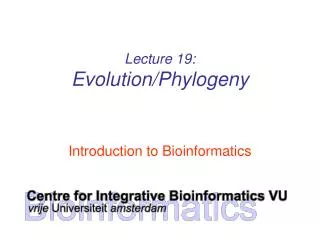
Lecture 19: Evolution/Phylogeny. Introduction to Bioinformatics. Bioinformatics. “Nothing in Biology makes sense except in the light of evolution” (Theodosius Dobzhansky (1900-1975)) “Nothing in bioinformatics makes sense except in the light of Biology”. Evolution.

E N D
Lecture 19:Evolution/Phylogeny Introduction to Bioinformatics
Bioinformatics • “Nothing in Biology makes sense except in the light of evolution” (Theodosius Dobzhansky (1900-1975)) • “Nothing in bioinformatics makes sense except in the light of Biology”
Evolution • Most of bioinformatics is comparative biology • Comparative biology is based upon evolutionary relationships between compared entities • Evolutionary relationships are normally depicted in a phylogenetic tree
Where can phylogeny be used • For example, finding out about orthology versus paralogy • Predicting secondary structure of RNA • Studying host-parasite relationships • Mapping cell-bound receptors onto their binding ligands • Multiple sequence alignment (e.g. Clustal)
Phylogenetic tree (unrooted) human Drosophila internal node fugu mouse leaf OTU – Observed taxonomic unit edge
Phylogenetic tree (unrooted) root human Drosophila internal node fugu mouse leaf OTU – Observed taxonomic unit edge
Phylogenetic tree (rooted) root time edge internal node (ancestor) leaf OTU – Observed taxonomic unit Drosophila human fugu mouse
How to root a tree m f • Outgroup – place root between distant sequence and rest group • Midpoint – place root at midpoint of longest path (sum of branches between any two OTUs) • Gene duplication – place root between paralogous gene copies h D f m h D 1 m f 3 1 2 4 2 3 1 1 1 h 5 D f m h D f- f- h- f- h- f- h- h-
Combinatoric explosion # sequences # unrooted # rooted trees trees 2 1 1 3 1 3 4 3 15 5 15 105 6 105 945 7 945 10,395 8 10,395 135,135 9 135,135 2,027,025 10 2,027,025 34,459,425
Tree distances Evolutionary (sequence distance) = sequence dissimilarity 5 human x mouse 6 x fugu 7 3 x Drosophila 14 10 9 x human 1 mouse 2 1 fugu 6 Drosophila mouse Drosophila human fugu
Phylogeny methods • Parsimony – fewest number of evolutionary events (mutations) – relatively often fails to reconstruct correct phylogeny, but methods have improved recently • Distance based – pairwise distances • Maximum likelihood – L = Pr[Data|Tree]
Parsimony & Distance parsimony Sequences 1 2 3 4 5 6 7 Drosophila t t a t t a a fugu a a t t t a a mouse a a a a a t a human a a a a a a t Drosophila mouse 1 6 4 5 2 3 7 human fugu distance human x mouse 2 x fugu 3 4 x Drosophila5 5 3 x Drosophila 2 mouse 1 2 1 1 human fugu mouse Drosophila human fugu
Maximum likelihood • If data=alignment, hypothesis = tree, and under a given evolutionary model, maximum likelihood selects the hypothesis (tree) that maximises the observed data • Extremely time consuming method • We also can test the relative fit to the tree of different models (Huelsenbeck & Rannala, 1997)
Bayesian methods • Calculates the posterior probability of a tree (Huelsenbeck et al., 2001) –- probability that tree is true tree given evolutionary model • Most computer intensive technique • Feasible thanks to Markov chain Monte Carlo (MCMC) numerical technique for integrating over probability distributions • Gives confidence number (posterior probability) per node
Distance methods: fastest • Clustering criterion using a distance matrix • Distance matrix filled with alignment scores (sequence identity, alignment scores, E-values, etc.) • Cluster criterion
Phylogenetic tree by Distance methods (Clustering) 1 2 3 4 5 Multiple alignment Similarity criterion Similarity matrix Scores 5×5 Phylogenetic tree
Human -KITVVGVGAVGMACAISILMKDLADELALVDVIEDKLKGEMMDLQHGSLFLRTPKIVSGKDYNVTANSKLVIITAGARQ Chicken -KISVVGVGAVGMACAISILMKDLADELTLVDVVEDKLKGEMMDLQHGSLFLKTPKITSGKDYSVTAHSKLVIVTAGARQ Dogfish –KITVVGVGAVGMACAISILMKDLADEVALVDVMEDKLKGEMMDLQHGSLFLHTAKIVSGKDYSVSAGSKLVVITAGARQ Lamprey SKVTIVGVGQVGMAAAISVLLRDLADELALVDVVEDRLKGEMMDLLHGSLFLKTAKIVADKDYSVTAGSRLVVVTAGARQ Barley TKISVIGAGNVGMAIAQTILTQNLADEIALVDALPDKLRGEALDLQHAAAFLPRVRI-SGTDAAVTKNSDLVIVTAGARQ Maizey casei -KVILVGDGAVGSSYAYAMVLQGIAQEIGIVDIFKDKTKGDAIDLSNALPFTSPKKIYSA-EYSDAKDADLVVITAGAPQ Bacillus TKVSVIGAGNVGMAIAQTILTRDLADEIALVDAVPDKLRGEMLDLQHAAAFLPRTRLVSGTDMSVTRGSDLVIVTAGARQ Lacto__ste -RVVVIGAGFVGASYVFALMNQGIADEIVLIDANESKAIGDAMDFNHGKVFAPKPVDIWHGDYDDCRDADLVVICAGANQ Lacto_plant QKVVLVGDGAVGSSYAFAMAQQGIAEEFVIVDVVKDRTKGDALDLEDAQAFTAPKKIYSG-EYSDCKDADLVVITAGAPQ Therma_mari MKIGIVGLGRVGSSTAFALLMKGFAREMVLIDVDKKRAEGDALDLIHGTPFTRRANIYAG-DYADLKGSDVVIVAAGVPQ Bifido -KLAVIGAGAVGSTLAFAAAQRGIAREIVLEDIAKERVEAEVLDMQHGSSFYPTVSIDGSDDPEICRDADMVVITAGPRQ Thermus_aqua MKVGIVGSGFVGSATAYALVLQGVAREVVLVDLDRKLAQAHAEDILHATPFAHPVWVRSGW-YEDLEGARVVIVAAGVAQ Mycoplasma -KIALIGAGNVGNSFLYAAMNQGLASEYGIIDINPDFADGNAFDFEDASASLPFPISVSRYEYKDLKDADFIVITAGRPQ Lactate dehydrogenase multiple alignment Distance Matrix 1 2 3 4 5 6 7 8 9 10 11 12 13 1 Human 0.000 0.112 0.128 0.202 0.378 0.346 0.530 0.551 0.512 0.524 0.528 0.635 0.637 2 Chicken 0.112 0.000 0.155 0.214 0.382 0.348 0.538 0.569 0.516 0.524 0.524 0.631 0.651 3 Dogfish 0.128 0.155 0.000 0.196 0.389 0.337 0.522 0.567 0.516 0.512 0.524 0.600 0.655 4 Lamprey 0.202 0.214 0.196 0.000 0.426 0.356 0.553 0.589 0.544 0.503 0.544 0.616 0.669 5 Barley 0.378 0.382 0.389 0.426 0.000 0.171 0.536 0.565 0.526 0.547 0.516 0.629 0.575 6 Maizey 0.346 0.348 0.337 0.356 0.171 0.000 0.557 0.563 0.538 0.555 0.518 0.643 0.587 7 Lacto_casei 0.530 0.538 0.522 0.553 0.536 0.557 0.000 0.518 0.208 0.445 0.561 0.526 0.501 8 Bacillus_stea 0.551 0.569 0.567 0.589 0.565 0.563 0.518 0.000 0.477 0.536 0.536 0.598 0.495 9 Lacto_plant 0.512 0.516 0.516 0.544 0.526 0.538 0.208 0.477 0.000 0.433 0.489 0.563 0.485 10 Therma_mari 0.524 0.524 0.512 0.503 0.547 0.555 0.445 0.536 0.433 0.000 0.532 0.405 0.598 11 Bifido 0.528 0.524 0.524 0.544 0.516 0.518 0.561 0.536 0.489 0.532 0.000 0.604 0.614 12 Thermus_aqua 0.635 0.631 0.600 0.616 0.629 0.643 0.526 0.598 0.563 0.405 0.604 0.000 0.641 13 Mycoplasma 0.637 0.651 0.655 0.669 0.575 0.587 0.501 0.495 0.485 0.598 0.614 0.641 0.000
Cluster analysis – (dis)similarity matrix C1 C2 C3 C4 C5 C6 .. 1 2 3 4 5 Raw table Similarity criterion Similarity matrix Scores 5×5 Di,j= (k | xik – xjk|r)1/r Minkowski metrics r = 2 Euclidean distance r = 1 City block distance
Cluster analysis – Clustering criteria Similarity matrix Scores 5×5 Cluster criterion Phylogenetic tree Single linkage - Nearest neighbour Complete linkage – Furthest neighbour Group averaging – UPGMA Ward Neighbour joining – global measure
Neighbour joining • Global measure – keeps total branch length minimal, tends to produce a tree with minimal total branch length • At each step, join two nodes such that distances are minimal (criterion of minimal evolution) • Agglomerative algorithm • Leads to unrooted tree
Neighbour joining y x x x y (c) (a) (b) x x x y y (f) (d) (e) At each step all possible ‘neighbour joinings’ are checked and the one corresponding to the minimal total tree length (calculated by adding all branch lengths) is taken.
How to assess confidence in tree • Bayesian method – time consuming • The Bayesian posterior probabilities (BPP) are assigned to internal branches in consensus tree • Bayesian Markov chain Monte Carlo (MCMC) analytical software such as MrBayes (Huelsenbeck and Ronquist, 2001) and BAMBE (Simon and Larget,1998) is now commonly used • Uses all the data • Distance method – bootstrap: • Select multiple alignment columns with replacement • Recalculate tree • Compare branches with original (target) tree • Repeat 100-1000 times, so calculate 100-1000 different trees • How often is branching (point between 3 nodes) preserved for each internal node? • Uses samples of the data
The Bootstrap 1 2 3 4 5 6 7 8 C C V K V I Y S M A V R L I F S M C L R L L F T 3 4 3 8 6 6 8 6 V K V S I I S I V R V S I I S I L R L T L L T L 5 1 2 3 Original 4 2x 3x 1 1 2 3 Non-supportive Scrambled 5