Download
1 / 64
690 likes | 1.04k Vues
Molecular Phylogeny and Evolution. Outline. Introduction to evolution and phylogeny Nomenclature of trees Five stages of molecular phylogeny: [1] selecting sequences [2] multiple sequence alignment [3] models of substitution [4] tree-building [5] tree evaluation.

E N D
Molecular Phylogeny and Evolution
Outline Introduction to evolution and phylogeny Nomenclature of trees Five stages of molecular phylogeny: [1] selecting sequences [2] multiple sequence alignment [3] models of substitution [4] tree-building [5] tree evaluation
Historical background Studies of molecular evolution began with the first sequencing of proteins, beginning in the 1950s. In 1953 Frederick Sanger and colleagues determined the primary amino acid sequence of insulin. (The accession number of human insulin is NP_000198) Page 219
Note the sequence divergence in the disulfide loop region of the A chain Fig. 7.3 Page 220
Historical background: insulin By the 1950s, it became clear that amino acid substitutions occur nonrandomly. For example, Sanger and colleagues noted that most amino acid changes in the insulin A chain are restricted to a disulfide loop region. Such differences are called “neutral” changes (Kimura, 1968; Jukes and Cantor, 1969). Subsequent studies at the DNA level showed that rate of nucleotide (and of amino acid) substitution is about six- to ten-fold higher in the C peptide, relative to the A and B chains. Page 219
0.1 x 10⁻⁹ 1 x 10⁻⁹ 0.1 x 10⁻⁹ Fig. 7.3 Page 220 Number of nucleotide substitutions/site/year
Historical background: insulin Surprisingly, insulin from the guinea pig (and from the related coypu) evolve seven times faster than insulin from other species. Why? The answer is that guinea pig and coypu insulin do not bind two zinc ions, while insulin molecules from most other species do. There was a relaxation on the structural constraints of these molecules, and so the genes diverged rapidly. Page 219
Guinea pig and coypu insulin have undergone an extremely rapid rate of evolutionary change Arrows indicate positions at which guinea pig insulin (A chain and B chain) differs from both human and mouse Fig. 7.3 Page 220
Molecular clock hypothesis In the 1960s, sequence data were accumulated for small, abundant proteins such as globins, cytochromes c, and fibrinopeptides. Some proteins appeared to evolve slowly, while others evolved rapidly. Linus Pauling, Emanuel Margoliash and others proposed the hypothesis of a molecular clock: For every given protein, the rate of molecular evolution is approximately constant in all evolutionary lineages Page 221
N 100 = 1 – e-(m/100) Molecular clock hypothesis As an example, Richard Dickerson (1971) plotted data from three protein families: cytochrome c, hemoglobin, and fibrinopeptides. The x-axis shows the divergence times of the species, estimated from paleontological data. The y-axis shows m, the corrected number of amino acid changes per 100 residues. n is the observed number of amino acid changes per 100 residues, and it is corrected to m to account for changes that occur but are not observed. Page 222
Molecular clock hypothesis: conclusions • Dickerson drew the following conclusions: • For each protein, the data lie on a straight line. Thus, • the rate of amino acid substitution has remained • constant for each protein. • The average rate of change differs for each protein. • The time for a 1% change to occur between two lines • of evolution is 20 MY (cytochrome c), 5.8 MY • (hemoglobin), and 1.1 MY (fibrinopeptides). • The observed variations in rate of change reflect • functional constraints imposed by natural selection. Page 223
Molecular clock for proteins: rate of substitutions per aa site per 109 years Fibrinopeptides 9.0 Kappa casein 3.3 Lactalbumin 2.7 Serum albumin 1.9 Lysozyme 0.98 Trypsin 0.59 Insulin 0.44 Cytochrome c 0.22 Histone H2B 0.09 Ubiquitin 0.010 Histone H4 0.010 Table 7-1 Page 223
Molecular clock hypothesis: implications If protein sequences evolve at constant rates, they can be used to estimate the times that sequences diverged. This is analogous to dating geological specimens by radioactive decay. Page 225
Molecular phylogeny: nomenclature of trees There are two main kinds of information inherent to any tree: topology and branch lengths. We will now describe the parts of a tree. Page 231
2 A F 1 1 G B 2 I H 2 C 1 D 6 E time Molecular phylogeny uses trees to depict evolutionary relationships among organisms. These trees are based upon DNA and protein sequence data. A 2 1 1 B 2 C 2 2 1 D 6 one unit E Fig. 7.8 Page 232
2 A F 1 1 G B 2 I H 2 C 1 D 6 E time Tree nomenclature operational taxonomic unit (OTU) such as a protein sequence taxon A 2 1 1 B 2 C 2 2 1 D 6 one unit E Fig. 7.8 Page 232
2 A F 1 1 G B 2 I H 2 C 1 D 6 E time Tree nomenclature Node (intersection or terminating point of two or more branches) branch (edge) A 2 1 1 B 2 C 2 2 1 D 6 one unit E Fig. 7.8 Page 232
2 A F 1 1 G B 2 I H 2 C 1 D 6 E time Tree nomenclature Branches are unscaled... Branches are scaled... A 2 1 1 B 2 C 2 2 1 D 6 one unit E …OTUs are neatly aligned, and nodes reflect time …branch lengths are proportional to number of amino acid changes Fig. 7.8 Page 232
2 A F 1 1 G B 2 I H 2 C 1 D 6 E time Tree nomenclature bifurcating internal node multifurcating internal node A 2 1 B 2 C 2 2 1 D 6 one unit E Fig. 7.9 Page 233
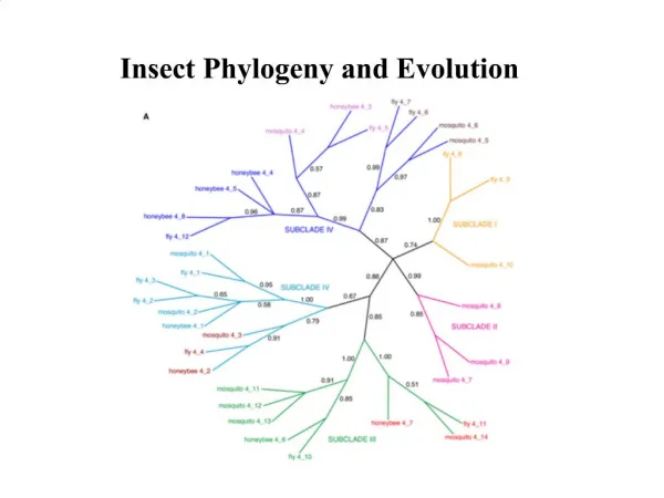
Examples of multifurcation: failure to resolve the branching order of some metazoans and protostomes Rokas A. et al., Animal Evolution and the Molecular Signature of Radiations Compressed in Time, Science 310:1933 (2005), Fig. 1.
Tree nomenclature: clades Clade ABF (monophyletic group) A 2 F 1 1 B G 2 I H 2 C 1 D 6 E time Fig. 7.8 Page 232
Tree nomenclature 2 A F 1 1 G B 2 I H 2 C Clade CDH 1 D 6 E time Fig. 7.8 Page 232
Tree nomenclature Clade ABF/CDH/G 2 A F 1 1 G B 2 I H 2 C 1 D 6 E time Fig. 7.8 Page 232
Examples of clades Lindblad-Toh et al., Nature 438: 803 (2005), fig. 10
Tree roots The root of a phylogenetic tree represents the common ancestor of the sequences. Some trees are unrooted, and thus do not specify the common ancestor. A tree can be rooted using an outgroup (that is, a taxon known to be distantly related from all other OTUs). Page 233
Tree nomenclature: roots past 9 1 5 7 8 6 7 8 2 3 present 4 2 6 4 5 3 1 Rooted tree (specifies evolutionary path) Unrooted tree Fig. 7.10 Page 234
Tree nomenclature: outgroup rooting past root 9 10 7 8 7 9 6 8 2 3 2 3 4 present 4 6 Outgroup (used to place the root) 5 1 5 1 Rooted tree Fig. 7.10 Page 234
Enumerating trees Cavalii-Sforza and Edwards (1967) derived the number of possible unrooted trees (NU) for n OTUs (n> 3): NU = The number of bifurcating rooted trees (NR) NR = For 10 OTUs (e.g. 10 DNA or protein sequences), the number of possible rooted trees is 34 million, and the number of unrooted trees is 2 million. Many tree-making algorithms can exhaustively examine every possible tree for up to ten to twelve sequences. (2n-5)! 2n-3(n-3)! (2n-3)! 2n-2(n-2)! Page 235
Numbers of possible trees extremely large for >10 sequences Number Number of Number of of OTUs rooted trees unrooted trees 2 1 1 3 3 1 4 15 3 5 105 15 10 34,459,425 105 20 8 x 10²¹ 2 x 10²⁰ Page 235
Five stages of phylogenetic analysis [1] Selection of sequences for analysis [2] Multiple sequence alignment [3] Selection of a substitution model [4] Tree building [5] Tree evaluation Page 243
Stage 1: Use of DNA, RNA, or protein For some phylogenetic studies, it may be preferable to use protein instead of DNA sequences. We saw that in pairwise alignment and in BLAST searching, protein is often more informative than DNA (Chapter 3). Page 240
Stage 1: Use of DNA, RNA, or protein For phylogeny, DNA can be more informative. --The protein-coding portion of DNA has synonymous and nonsynonymous substitutions. Thus, some DNA changes do not have corresponding protein changes. Page 240
Stage 1: Use of DNA, RNA, or protein For phylogeny, DNA can be more informative. --The protein-coding portion of DNA has synonymous and nonsynonymous substitutions. Thus, some DNA changes do not have corresponding protein changes. If the synonymous substitution rate (dS) is greater than the nonsynonymous substitution rate (dN), the DNA sequence is under negative (purifying) selection. This limits change in the sequence (e.g. insulin A chain). If dS < dN, positive selection occurs. For example, a duplicated gene may evolve rapidly to assume new functions. Page 230
Stage 1: Use of DNA, RNA, or protein For phylogeny, DNA can be more informative. --Some substitutions in a DNA sequence alignment can be directly observed: single nucleotide substitutions, sequential substitutions, coincidental substitutions. Page 241
Stage 1: Use of DNA, RNA, or protein For phylogeny, DNA can be more informative. --Noncoding regions (such as 5’ and 3’ untranslated regions) may be analyzed using molecular phylogeny. --Pseudogenes (nonfunctional genes) are studied by molecular phylogeny --Rates of transitions and transversions can be measured. Transitions: purine (A G) or pyrimidine (C T) substitutions Transversion: purine pyrimidine Page 242
Stage 1: Use of DNA, RNA, or protein For phylogeny, protein sequences are also often used. --Proteins have 20 states (amino acids) instead of only four for DNA, so there is a stronger phylogenetic signal. Nucleotides are unordered characters: any one nucleotide can change to any other in one step. An ordered character must pass through one or more intermediate states before reaching the final state. Amino acid sequences are partially ordered character states: there is a variable number of states between the starting value and the final value. Page 243
Five stages of phylogenetic analysis [1] Selection of sequences for analysis [2] Multiple sequence alignment [3] Selection of a substitution model [4] Tree building [5] Tree evaluation Page 244
Stage 2: Multiple sequence alignment The fundamental basis of a phylogenetic tree is a multiple sequence alignment. (If there is a misalignment, or if a nonhomologous sequence is included in the alignment, it will still be possible to generate a tree.) Consider the following alignment of orthologous globins (see Fig. 3.2) Page 244
Stage 2: Multiple sequence alignment [1] Confirm that all sequences are homologous [2] Adjust gap creation and extension penalties as needed to optimize the alignment [3] Restrict phylogenetic analysis to regions of the multiple sequence alignment for which data are available for all taxa (delete columns having incomplete data or gaps). Page 244
Five stages of phylogenetic analysis [1] Selection of sequences for analysis [2] Multiple sequence alignment [3] Selection of a substitution model [4] Tree building [5] Tree evaluation Page 246
Stage 4: Tree-building methods: distance The simplest approach to measuring distances between sequences is to align pairs of sequences, and then to count the number of differences. The degree of divergence is called the Hamming distance. For an alignment of length N with n sites at which there are differences, the degree of divergence D is: D = n / N But observed differences do not equal genetic distance! Genetic distance involves mutations that are not observed directly. Page 247
Stage 4: Tree-building methods Distance-based methods involve a distance metric, such as the number of amino acid changes between the sequences, or a distance score. Examples of distance-based algorithms are UPGMA and neighbor-joining. Character-based methods include maximum parsimony and maximum likelihood. Parsimony analysis involves the search for the tree with the fewest amino acid (or nucleotide) changes that account for the observed differences between taxa. Page 254
Stage 4: Tree-building methods We can introduce distance-based and character-based tree-building methods by referring to a group of orthologous globin proteins. Page 255
Stage 4: Tree-building methods [1] distance-based [2] character-based: maximum parsimony
1 2 3 4 5 Tree-building methods: UPGMA UPGMA is unweighted pair group method using arithmetic mean Fig. 7.26 Page 257
1 2 3 4 5 Tree-building methods: UPGMA Step 1: compute the pairwise distances of all the proteins. Get ready to put the numbers 1-5 at the bottom of your new tree. Fig. 7.26 Page 257
1 2 3 4 5 Tree-building methods: UPGMA Step 2: Find the two proteins with the smallest pairwise distance. Cluster them. 6 1 2 Fig. 7.26 Page 257
1 2 3 4 5 Tree-building methods: UPGMA Step 3: Do it again. Find the next two proteins with the smallest pairwise distance. Cluster them. 6 7 1 2 4 5 Fig. 7.26 Page 257
1 2 3 4 5 Tree-building methods: UPGMA Step 4: Keep going. Cluster. 8 7 6 3 1 2 4 5 Fig. 7.26 Page 257
1 2 3 4 5 Tree-building methods: UPGMA Step 4: Last cluster! This is your tree. 9 8 7 6 1 2 4 5 3 Fig. 7.26 Page 257