Introduction to Data Management and Analysis in Stata
This session covers essential commands and techniques for data management and analysis in Stata. We explore navigating directories, storing commands, creating and saving do-files, and using the data editor. Key table display commands such as `tabulate`, `tabstat`, and `table` are introduced to summarize and analyze data effectively. Using Rosner's forced expiration volume dataset, we demonstrate how to label variables, create categorical data, and identify associations between variables. Learn to structure your data efficiently using long and wide formats.

Introduction to Data Management and Analysis in Stata
E N D
Presentation Transcript
Tables, Long data, Frequency weighting, String data
Key points from our first session: Where are you? cd Navigate to a directory cd Change from your current directory cd What files are in the current directory? dir How do you store commands? do file Where is your do file? with the data How do you create a do file? do editor How do you save a do file? do editor … save Name your variables to clarify their purpose Label the values of your categorical variables to clarify their significance Use the use command with the clear option to load a dataset Use the save command with the replace option to save a dataset
Key points from our first session (cont.): Use the data editor to check your variables Use the do-file editor to edit, or run do files Data editor Do-file editor Variables Passed commands Results
Tables Stata supports the following table display commands table, tabdisp, tabstat, tabsum, tabulate …. to capture trends and patterns in data We will again explore each of these interactively
USE tabulate (tab) to display simple summaries, relative cell counts, associative measures between row and column variables USE table to display statistics concerning variables in a table and to gain control of the table layout, for publication purposes USE tabstat to display the (same comprehensive array of) statistics of (several) variables in a table and to gain control of the table layout, for publication purposes, when only one classifying (categorical) variable is considered USE tabdisp to display your own calculations, and observations, in a table in which you do not want any special treatment of the numbers
Rosner’s dataset, ‘fev.dat’ relates to forced expiration volumes of children of different age, sex, height, to smoking exposure. We’ll ‘use’ the data, ‘label’ the variables, and make a ‘table’ … what’s in this table?: use fev, clear summarize label def slabel 1 Male 0 Female label def mlabel 1 Smoker 0 "Non-smoker" label val smoke mlabel label val sex slabel table smoke sex, c(mean age p50 age) row col format(%7.2f) Unfortunately age is an interval variable so we’ll make a categorical variable from it and explore the consequences also using tables. xtile q_age=age, n(5) table sex q_age, c(m age p50 age freq) format(%7.2f) table q_age smoke sex, format(%7.2f) row col scol We’ll now see what ‘tabstat’ can provide for us with this data tabstat age, by(sex) s(mean p50 range sd sem) format(%7.2f) Is there an association between age-group, and smoking exposure? tabulate smoke q_age, chi ex row col
Output from some of the Table commands . xtile q_age=age, n(5) . table sex q_age, c(m age p50 age freq) format(%7.2f) --------------------------------------------- | 5 quantiles of age sex | 1 2 3 4 5 ----------+---------------------------------- Female | 6.83 9.00 10.57 12.00 14.42 | 7.00 9.00 11.00 12.00 14.00 | 111 44 79 29 55 | Male | 6.77 9.00 10.49 12.00 14.68 | 7.00 9.00 10.00 12.00 14.00 | 104 50 92 28 62 --------------------------------------------- . tabstat age, by(sex) s(mean p50 range sd sem) format(%7.2f) Summary for variables: age by categories of: sex sex | mean p50 range sd se(mean) -------+-------------------------------------------------- Female | 9.84 10.00 16.00 2.93 0.16 Male | 10.01 10.00 16.00 2.98 0.16 -------+-------------------------------------------------- Total | 9.93 10.00 16.00 2.95 0.12 ----------------------------------------------------------
. table q_age smoke sex, format(%7.2f) row col scol ------------------------------------------------------------------------------------ 5 | sex and smoke quantiles | ------------- Female ------------- -------------- Male -------------- of age | Non-smoker Smoker Total Non-smoker Smoker Total ----------+------------------------------------------------------------------------- 1 | 111 111 104 104 2 | 44 44 49 1 50 3 | 69 10 79 88 4 92 4 | 25 4 29 25 3 28 5 | 30 25 55 44 18 62 | Total | 279 39 318 310 26 336 ------------------------------------------------------------------------------------ ---------------------------------------------- 5 | sex and smoke quantiles | -------------- Total ------------- of age | Non-smoker Smoker Total ----------+----------------------------------- 1 | 215 215 ... 2 | 93 1 94 3 | 157 14 171 4 | 50 7 57 5 | 74 43 117 | Total | 589 65 654 ----------------------------------------------
Long data … and Wide data Long data: Involves multiple instances (data rows) of each subject Is a natural organization of data for statistical analysis Involves variables with a single purpose Is usually an inefficient organization for data entry Wide data: Is compact Involves a single instance (data row) of each subject Is very efficient for data entry Can easily exposes patterns in the data at a glance Is NOT a natural organization for data analysis It is extremely easy to convert long data to wide data and vice versa. This will be the topic of a future class
. use "long data", clear . describe Contains data from long data.dta obs: 532 vars: 5 27 Jan 2004 17:04 size: 9,044 (99.9% of memory free) ---------------------------------------------------------------- storage display value variable name type format label variable label ---------------------------------------------------------------- time int %8.0g subject int %8.0g day byte %8.0g Day glucose float %9.0g Glucose insulin float %9.0g Insulin ---------------------------------------------------------------- Sorted by: . table subject day ---------------------- | Day subject | -10 28 ----------+----------- 2474 | 14 14 2511 | 14 14 2542 | 14 14 2636 | 14 14 2638 | 14 14 2681 | 14 14 2687 | 14 14 2744 | 14 14 2805 | 14 14 2818 | 14 14 2822 | 14 14 2832 | 14 14 2885 | 14 14 2904 | 14 14 2927 | 14 14 2935 | 14 14 2939 | 14 14 2976 | 14 14 2994 | 14 14 ---------------------- Here we ‘describe’ a long dataset involving the application of the FSIGT on a number of subjects; each subject received 2 diets (treatment) Tables are probably the best way of describing, or understanding the nature of a long dataset Here it appears that there are NOT the same number of replicates across treatments by subjects
collapse -ing the data to means provides a convenient way of getting the data into a more regular form collapse glucose insulin, by(subject time day) Now, using tables and graphs we can review patterns in our long data table subject day scatter glucose time, c(L L) s(i i) sort(subject time) by(day) In order to widen our data with reshape we can’t have –ve times recode time –15=1500 recode day -10=10 To make the long data wide we perform 2 reshapes, the first appends treatment to the variable names, and the second appends time to the name. reshape wide glucose insulin, i(time subject) j(day) reshape wide gluc* ins*, i(subject) j(time)
glucose1030 float %9.0g 30 glucose10 insulin1030 float %9.0g 30 insulin10 glucose2830 float %9.0g 30 glucose28 insulin2830 float %9.0g 30 insulin28 glucose1045 float %9.0g 45 glucose10 insulin1045 float %9.0g 45 insulin10 glucose2845 float %9.0g 45 glucose28 insulin2845 float %9.0g 45 insulin28 glucose1060 float %9.0g 60 glucose10 insulin1060 float %9.0g 60 insulin10 glucose2860 float %9.0g 60 glucose28 insulin2860 float %9.0g 60 insulin28 glucose1090 float %9.0g 90 glucose10 insulin1090 float %9.0g 90 insulin10 glucose2890 float %9.0g 90 glucose28 insulin2890 float %9.0g 90 insulin28 glucose10120 float %9.0g 120 glucose10 insulin10120 float %9.0g 120 insulin10 glucose28120 float %9.0g 120 glucose28 insulin28120 float %9.0g 120 insulin28 glucose10150 float %9.0g 150 glucose10 insulin10150 float %9.0g 150 insulin10 glucose28150 float %9.0g 150 glucose28 insulin28150 float %9.0g 150 insulin28 glucose10180 float %9.0g 180 glucose10 insulin10180 float %9.0g 180 insulin10 glucose28180 float %9.0g 180 glucose28 insulin28180 float %9.0g 180 insulin28 glucose101500 float %9.0g 1500 glucose10 insulin101500 float %9.0g 1500 insulin10 glucose281500 float %9.0g 1500 glucose28 insulin281500 float %9.0g 1500 insulin28 ------------------------------------------------------------ Sorted by: subject Now our wide data has the following characteristics . describe Contains data obs: 19 vars: 57 size: 4,370 (99.9% of memory free) ------------------------------------------------------------ storage display value variable name type format label variable label ------------------------------------------------------------ subject int %8.0g glucose100 float %9.0g 0 glucose10 insulin100 float %9.0g 0 insulin10 glucose280 float %9.0g 0 glucose28 insulin280 float %9.0g 0 insulin28 glucose105 float %9.0g 5 glucose10 insulin105 float %9.0g 5 insulin10 glucose285 float %9.0g 5 glucose28 insulin285 float %9.0g 5 insulin28 glucose1010 float %9.0g 10 glucose10 insulin1010 float %9.0g 10 insulin10 glucose2810 float %9.0g 10 glucose28 insulin2810 float %9.0g 10 insulin28 glucose1015 float %9.0g 15 glucose10 insulin1015 float %9.0g 15 insulin10 glucose2815 float %9.0g 15 glucose28 insulin2815 float %9.0g 15 insulin28 glucose1020 float %9.0g 20 glucose10 insulin1020 float %9.0g 20 insulin10 glucose2820 float %9.0g 20 glucose28 insulin2820 float %9.0g 20 insulin28 glucose1025 float %9.0g 25 glucose10 insulin1025 float %9.0g 25 insulin10 glucose2825 float %9.0g 25 glucose28 insulin2825 float %9.0g 25 insulin28
Description of the long data organization . describe Contains data obs: 532 vars: 5 27 Jan 2004 17:04 size: 9,044 (99.9% of memory free) --------------------------------------------------------------- Description of the wide data organization Contains data obs: 19 vars: 57 size: 4,370 (99.9% of memory free) ---------------------------------------------------------------
Another Rosner dataset relates to the use of two blood pressure lowering drugs Nifedipine and Propanolol in a heart rate lowering experiment, see Rosner (dataset descriptions) . use nifed, clear . describe Contains data from nifed.dta obs: 34 vars: 10 26 Nov 1997 17:13 size: 748 (99.9% of memory free) ------------------------------------------------------------------- storage display value variable name type format label variable label ------------------------------------------------------------------- id byte %9.0g grp str1 %9s bhr int %9.0g hr1 int %9.0g hr2 int %9.0g hr3 int %9.0g bsp int %9.0g sbp1 int %9.0g sbp2 int %9.0g sbp3 int %9.0g ------------------------------------------------------------------- . list +-------------------------------------------------------------+ | id grp bhr hr1 hr2 hr3 bsp sbp1 sbp2 sbp3 | |-------------------------------------------------------------| 1. | 1 P 60 70 64 128 110 120 . . | 2. | 2 N 52 64 98 180 156 160 140 . | 3. | 3 P 100 94 190 140 . . . . | 4. | 4 N 84 88 96 112 136 126 122 110 | 5. | 5 P 56 70 61 64 230 150 130 150 | |-------------------------------------------------------------| 6. | 6 P 105 120 142 150 . . . . | .... Here we use, describe, and list the data in Rosner’s nifed dataset.
. rename bhr hr0 . rename bsp sbp0 . reshape long sbp hr, i(id grp) j(rep) (note: j = 0 1 2 3) Data wide -> long ---------------------------------------------------- Number of obs. 34 -> 136 Number of variables 10 -> 5 j variable (4 values) -> rep xij variables: sbp0 sbp1 ... sbp3 -> sbp hr0 hr1 ... hr3 -> hr ---------------------------------------------------- Following the sequence of commands shown here we create a long version of this data Here we describe the data, now in long form . describe Contains data obs: 136 vars: 5 size: 1,496 (99.9% of memory free) ------------------------------------------------------------ storage display value variable name type format label variable label ------------------------------------------------------------ id byte %9.0g grp str1 %9s rep byte %9.0g hr int %9.0g sbp int %9.0g ------------------------------------------------------------
P P N P P N N N #d ; collapse hr sbp, by(rep grp); scatter sbp hr rep, c(L L) mlabel(grp grp) sort(grp rep) clw(thick thick) clp(dash dot) title("Nifedipine - Propanalol Study") xtitle(Replication Number) ylabel(,angle(0)); Here we illustrate the drug effects with application wrt heart rate and blood pressure Nifedipine - Propanalol Study 160 140 N N 120 P 100 P 80 P N P N 0 1 2 3 Replication Number (mean) sbp (mean) hr
Frequency weighting . use "CHD Example", clear . label define blabel 0 "< 160" 1 ">=160" . label define clabel 0 " No CHD" 1 CHD . label value Blood_pressure blabel . label value CHD clabel . label var count Count . list +---------------------------+ | Blood_~e CHD count | |---------------------------| 1. | >=160 CHD 95 | 2. | < 160 CHD 173 | 3. | >=160 No CHD 201 | 4. | < 160 No CHD 894 | +---------------------------+ . Summarize Blood_pressure CHD Variable | Obs Mean Std. Dev. Min Max -------------+-------------------------------------------------------- Blood_pres~e | 4 .5 .5773503 0 1 CHD | 4 .5 .5773503 0 1 . summarize Blood_pressure CHD [fwe=count] Variable | Obs Mean Std. Dev. Min Max -------------+-------------------------------------------------------- Blood_pres~e | 1363 .217168 .4124693 0 1 CHD | 1363 .1966251 .3975923 0 1 Why do summarize and frequency weighted summarize produce different results?
Frequency weighting …. Unweighted: mean x = Sum of [x’s] /Number of [x’s] for CHD = 2/4 = 0.5 Weighted: mean x = Sum of [x’s*frequencies] /Sum of [frequencies] for CHD = [1*95 + 1*173 + 0*201 + 0*894]/[95 + 173 + 201 + 894] = . di [95 + 173]/[95 + 173 + 201 + 894] = 0.19662509 What would we expect for Blood_pressure
Frequency weighting In mathematical formalism we write Here xi is the ith value of x, and fi is the frequency that the ith value of x occurs in the dataset
String data Strings are sequences of letters and numbers “men”, “women”, “survived”, “lost to follow-up”, “Jan:27:2004” A sequence of numbers can be a string depending on the circumstances “1.23”, “-200.99”, “2” No numerical manipulation can be performed on a string It is quite simple to: Recognize strings codebook, describe Convert strings to numerics encode, real, destring Convert numerics to strings decode, string Use strings in a numeric sense xi
Create a string form of CHD, dCHD, and examine the new variable . decode CHD, gen(dCHD) . summarize dCHD Variable | Obs Mean Std. Dev. Min Max -------------+-------------------------------------------------------- dCHD | 0 . summarize dCHD [fwe=count] Variable | Obs Mean Std. Dev. Min Max -------------+-------------------------------------------------------- dCHD | 0 . describe dCHD storage display value variable name type format label variable label ---------------------------------------------------------------------- dCHD str7 %9s . codebook dCHD ---------------------------------------------------------------------- dCHD ---------------------------------------------------------------------- type: string (str7) unique values: 2 missing "": 0/4 tabulation: Freq. Value 2 "No CHD" 2 "CHD" warning: variable has leading and embedded blanks
The ‘xi’ modifier creates a unique series of indicator variables which, in a sense, allow the categoric variable to be ‘numerically’ manipulated . xi: summarize i.dCHD [fwe=count] i.dCHD _IdCHD_1-2 (_IdCHD_1 for dCHD==No CHD omitted) Variable | Obs Mean Std. Dev. Min Max -------------+-------------------------------------------------------- _IdCHD_2 | 1363 .1966251 .3975923 0 1 . list +------------------------------------------------+ | Blood_~e CHD count dCHD _IdCHD_2 | |------------------------------------------------| 1. | >=160 CHD 95 CHD 1 | 2. | < 160 CHD 173 CHD 1 | 3. | >=160 No CHD 201 No CHD 0 | 4. | < 160 No CHD 894 No CHD 0 | +------------------------------------------------+
Using the ‘char’ utility we can control the ‘referent’ state of a categoric variable . char dCHD [omit] "CHD" . char list dCHD[omit]: CHD . list +------------------------------------------------+ | Blood_~e CHD count dCHD _IdCHD_2 | |------------------------------------------------| 1. | >=160 CHD 95 CHD 1 | 2. | < 160 CHD 173 CHD 1 | 3. | >=160 No CHD 201 No CHD 0 | 4. | < 160 No CHD 894 No CHD 0 | +------------------------------------------------+ . xi: summarize i.dCHD [fwe=count] i.dCHD _IdCHD_1-2 (_IdCHD_2 for dCHD==CHD omitted) Variable | Obs Mean Std. Dev. Min Max -------------+-------------------------------------------------------- _IdCHD_1 | 1363 .8033749 .3975923 0 1 Note that we now computer the complimentary probability with the frequency weighted summarize
To restore the omitted state of a categoric variable to its default state . char list _IdCHD_2 . char dCHD [omit] . char list _IdCHD_1