BRAVO Back-Trajectory Analyses
BRAVO Back-Trajectory Analyses. BRAVO Meeting, San Antonio, TX, 23 March 2001. Why Consider ATAD? History of use at Big Bend - How Good is our past? History of comparison to other wind fields. ATAD vs Hysplit with EDAS & FNL Wind Fields

BRAVO Back-Trajectory Analyses
E N D
Presentation Transcript
BRAVO Back-Trajectory Analyses BRAVO Meeting, San Antonio, TX, 23 March 2001 Why Consider ATAD? History of use at Big Bend - How Good is our past? History of comparison to other wind fields. ATAD vs Hysplit with EDAS & FNL Wind Fields How different are they and why Results of preliminary qualitative back-trajectory analyses.
How are ATAD and Hysplit Different? 1. Input data Raw sounding data for ATAD Modeled EDAS or FNL wind fields for Hysplit 2. Length of time data is obtainable 1946 - present for ATAD 1997 - present for Hysplit 3. Model methodology Average wind in a transport layer and radius for ATAD “Data following” for Hysplit (other options also) 4. Frequency of Output 4 starts/day, endpoints 8 times/day for ATAD, 5 day max length hourly starts, hourly endpoints for Hysplit, max length > 10 days
ATAD Methodology from Heffter, 1980
EDAS Meteorological Data Archive The EDAS (Eta Data Assimilation System) data are a product of the NWS' National Centers for Environmental Prediction (NCEP). EDAS is a data assimilation system consisting of successive 3-h Eta model forecasts and Optimum Interpolation (OI) analyses. • 79 by 55 Lambert Conformal grid ~ 80 km resolution. • 22 vertical layers on constant pressure surfaces from 1000 to 50 mbar • 3 hour time increment • Upper Air Data: 3-D winds, Temp, RH • Surface Data includes: pressure, 10 meter winds, 2 meter Temp & RH, Momentum and heat flux • Data is available from 1/97 to present. Note Oct. 1999 data is unavailable due to a fire at NCEP
FNL Meteorological Data Archive The FNL data is a product of the Global Data Assimilation System (GDAS), which uses the Global spectral Medium Range Forecast model (MRF) to assimilate multiple sources of measured data and forecast meteorology. • 129 x 129 Polar Stereographic Grid with ~ 190 km resolution. • 12 vertical layers on constant pressure surfaces from 1000 to 50 mbar • 6 hour time increment • Upper Air Data: 3-D winds, Temp, RH • Surface Data includes: pressure, 10 meter winds, 2 meter Temp & RH, Momentum and heat flux • Data is available from 1/97 to present.
ATAD vs Hysplit…How Different Can They Be? Well, at times, pretty different!
A common pattern in July & Aug... Atad most southerly, EDAS most easterly with FNL in between. 7/18-7/28, first few days in August, and end of August
Height Differences Between EDAS & FNL can be large - even on order of Km
Directional Differences Between EDAS & FNL can be large (See 1000m traj.)
Even When Heights match, Directions can Differ Between EDAS & FNL (See 2000 m)
Overall Residence Time June - September, 1999 ATAD, EDAS, FNL
2 Wind Fields and 2 Heights
Correlations between Overall Residence Times 3-Day Trajectories June-Sep 1999 atad EDAS2000 EDAS1000 EDAS100 EDAS10 FNL2000 FNL1000 FNL100 FNL10 atad 1.000 0.732 0.769 0.648 0.662 0.790 0.806 0.653 0.644 EDAS2000 0.732 1.000 0.878 0.753 0.787 0.962 0.811 0.714 0.730 EDAS1000 0.769 0.878 1.000 0.942 0.945 0.903 0.956 0.933 0.927 EDAS100 0.648 0.753 0.942 1.000 0.994 0.780 0.870 0.973 0.986 EDAS10 0.662 0.787 0.945 0.994 1.000 0.812 0.867 0.955 0.977 FNL2000 0.790 0.962 0.903 0.780 0.812 1.000 0.860 0.751 0.762 FNL1000 0.806 0.811 0.956 0.870 0.867 0.860 1.000 0.893 0.866 FNL100 0.653 0.714 0.933 0.973 0.955 0.751 0.893 1.000 0.989 FNL10 0.644 0.730 0.927 0.986 0.977 0.762 0.866 0.989 1.000
Which is “Right”? Why? Does it Matter? 1. Transport heights matter. ATAD “transport layer” vs Hysplit vertical wind speed driven transport height. To do “standard” residence time analyses with Hysplit may require 3-D analysis. 2. Tracer concentrations should help on days with large differences. 3. MM5 Winds should help. 4. Qualitative results for some residence-time-type analyses suggest similar results no matter which is used.
TX/MX Border Maybe Not Real E. Texas TX/MX Border with ATAD saying Mexico
Example of ATAD saying Mexico while Hysplit is along the border.
High Concentration Source Contribution Function for CSU Sulfate Ion, July-Oct, ATAD, EDAS & FNL started at 1000 m.
What’s Next? 1. To use Hysplit in the “usual” ATAD residence time-type analyses requires some consideration of trajectory height. 3-D residence time? 2. If ATAD’s directions are wrong, choices….. Modify ATAD to use EDAS and/or FNL winds Switch to Hysplit with some height consideration. Abandon ATAD in favor of Monte Carlo model 3. Further analyses of BRAVO data, measured sfc & upper air winds, tracer, MM5 winds, spatial patterns in chem data should all help in deciding which model to use and why. 4. Continue with analyses of other species and other types of trajectory-based analyses.